East Africa Unveiled

Name and Description of the dataset used in this blog.

• Name: Global Country Information Dataset 2023 (last update 4 months ago)

A Comprehensive Dataset Empowering In-Depth Analysis and Cross-Country Insights

link: https://www.kaggle.com/datasets/nelgiriyewithana/countries-of-the-world-2023

• Description

This comprehensive dataset provides a wealth of information about all countries worldwide, covering a wide range of indicators and attributes. It encompasses demographic statistics, economic indicators, environmental factors, healthcare metrics, education statistics, and much more. With every country represented, this dataset offers a complete global perspective on various aspects of nations, enabling in-depth analyses and cross-country comparisons.

• My focus is on East Africa Countries

Introduction

East Africa, a region characterized by its diverse landscapes, rich cultural heritage, and dynamic socio-economic status. This dataset allows us to delve into the intricate details of East African countries, providing a holistic understanding of their demographic, economic, environmental, and healthcare landscapes. With a spotlight on key variables such as population density, economic indicators, healthcare metrics, and more, we aim to paint a vivid picture of the East African nations and facilitate insightful cross-country comparisons.

Encompassing countries like Kenya, Tanzania, Uganda, Rwanda, Burundi, and South Sudan, the East African region is home to a tapestry of cultures, languages, and historical narratives. As I embark on this descriptive and visualization journey, I will leverage the wealth of information within the dataset to unravel the intricacies of each nation. From the bustling cities to the vast agricultural lands, from economic indicators shaping the growth trajectory to healthcare metrics influencing public well-being, our analysis aims to provide a nuanced understanding of East Africa. Lets get started

Code

library(tidyverse)
library(scales)
world <- read.csv("world-data-2023.csv")
east_africa <- world %>% filter(Country %in% c("Kenya", "Uganda","Tanzania",
                 "South Sudan","Rwanda","Burundi"))

Population density

Code

east_africa %>% ggplot(aes(Country, as.numeric(Density..P.Km2.), fill = Country, label = Density..P.Km2.))+geom_col()+
  geom_text(vjust = -0.2)+
  labs(title = "Population density measured in persons per square kilometer",
       y = "Density (P/Km2)",
       caption = "Data source:Kaggle")+
  theme(axis.text.x = element_text(angle = 45, face = "bold"),legend.position = "none")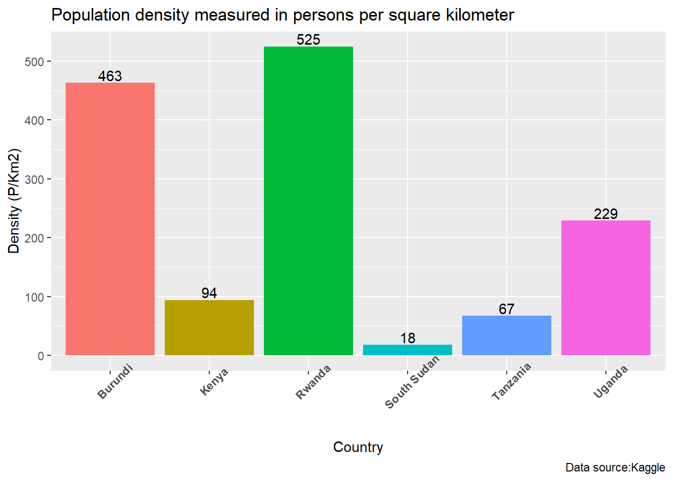

Regions with high population density often indicate crowded areas or areas with limited available land.Population density information is crucial for policymakers to plan for infrastructure development, housing, healthcare facilities, and other essential services.It helps in formulating strategies to manage urbanization, ensuring sustainable development and improving the overall quality of life for residents. Rwanda and Burundi high population density can be attributed to limited available land. South sudan population is relatively sparse and is most concentrated in refuge zone.

Agricultural Land (%)

Code

east_africa %>% ggplot(aes(Country, Agricultural.Land...., fill = Country, label = Agricultural.Land....))+geom_col()+
  geom_text(vjust = -0.2)+
  labs(title = "Percentage of land area used for agricultural purposes",
       y = "Agricultural.Land",
       caption = "Data source:Kaggle")+
  theme(axis.text.x = element_text(angle = 45, face = "bold"),legend.position = "none")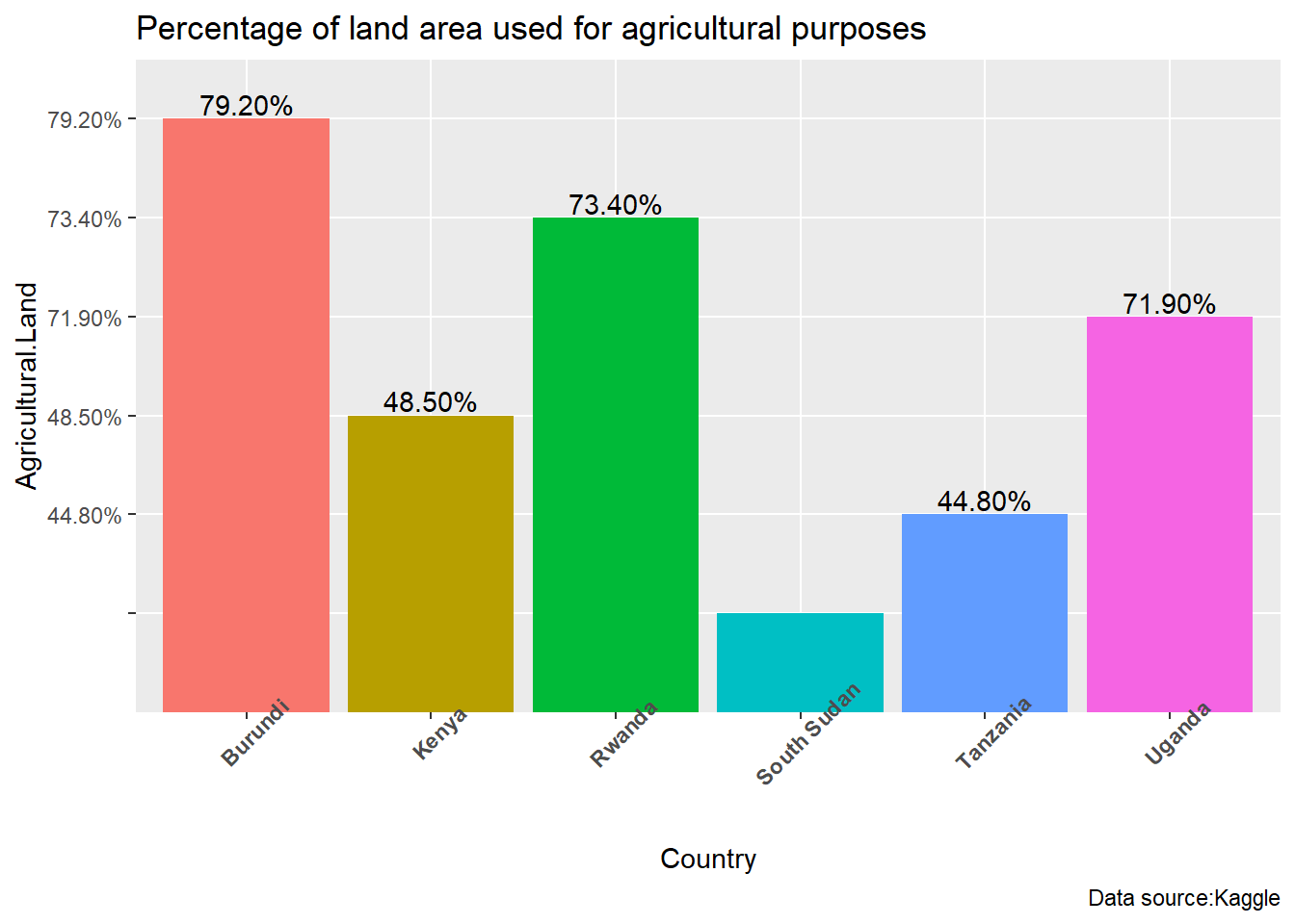

A higher percentage of land allocated to agriculture often indicates the economic significance of the agricultural sector within a country. Countries with a substantial portion of their land dedicated to agriculture may have economies heavily reliant on farming activities agriculture land is directly linked to domestic food security. Most of the economy of Eat Africa are heavly reliant of Agriculture.

Land Area (Km2)

Code

east_africa %>% ggplot(aes(Country,as.numeric(gsub(",","",Land.Area.Km2.)), fill = Country, label = Land.Area.Km2.))+geom_col()+
  geom_text(vjust = -0.2)+
  labs(title = "Total land area of the country in square kilometers.",
       y = "Land.Area.Km2",
       caption = "Data source:Kaggle")+
  theme(axis.text.x = element_text(angle = 45, face = "bold"),legend.position = "none")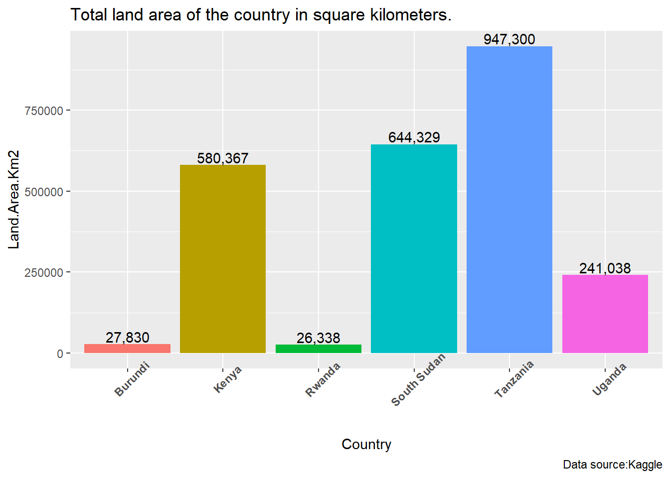

Land area refers to the total extent of a geographical area measured in square kilometers.Countries with large land areas may have more diverse ecosystems and potential resource abundance.

Armed Forces Size

Code

east_africa %>% ggplot(aes(Country,as.numeric(gsub(",","",Armed.Forces.size )), fill = Country, label = Armed.Forces.size ))+geom_col()+
  geom_text(vjust = -0.2)+
  labs(title = "Size of the armed forces in the country.",
       y = "Armed.Forces.size ",
       caption = "Data source:Kaggle")+
  theme(axis.text.x = element_text(angle = 45, face = "bold"),legend.position = "none")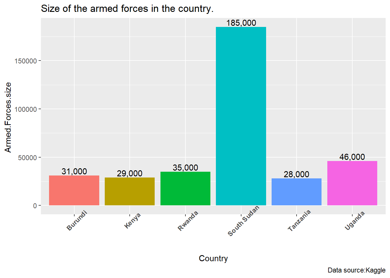

Armed forces size refers to the total number of active military personnel, including the army, navy, air force, and other branches. It encompasses both professional soldiers and conscripted individuals, providing a comprehensive view of a country’s military manpower.the size of armed forces is critical for nation’s defense strategy and is determined by 1)Population Size: The need to maintain internal security and territorial integrity in a densely populated nation may drive the requirement for a larger military force. 2)Geopolitical Context: geopolitical position might contribute to the need for a larger military. 3)Historical Factors: Historical events, such as conflicts, wars, or periods of instability, can shape the size and structure of a country’s military. 4)Economic Considerations: Economic factors, such as the ability to allocate resources to defense, play a significant role in determining the size and capabilities of a military. 5)Security Challenges: security challenges, including insurgencies, terrorism, and ethno-religious conflicts may necessitate a larger military to address various security threats. 6)Resource Allocation: The decision on the size of the military is influenced by how a country allocates its resources among competing needs.

Birth Rate

Code

east_africa %>% ggplot(aes(Country, Birth.Rate, fill = Country, label =  Birth.Rate ))+geom_col()+
  geom_text(vjust = -0.2)+
  labs(title = "Number of births per 1,000 population per year.",
       y = " Birth.Rate",
       caption = "Data source:Kaggle")+
  theme(axis.text.x = element_text(angle = 45, face = "bold"),legend.position = "none")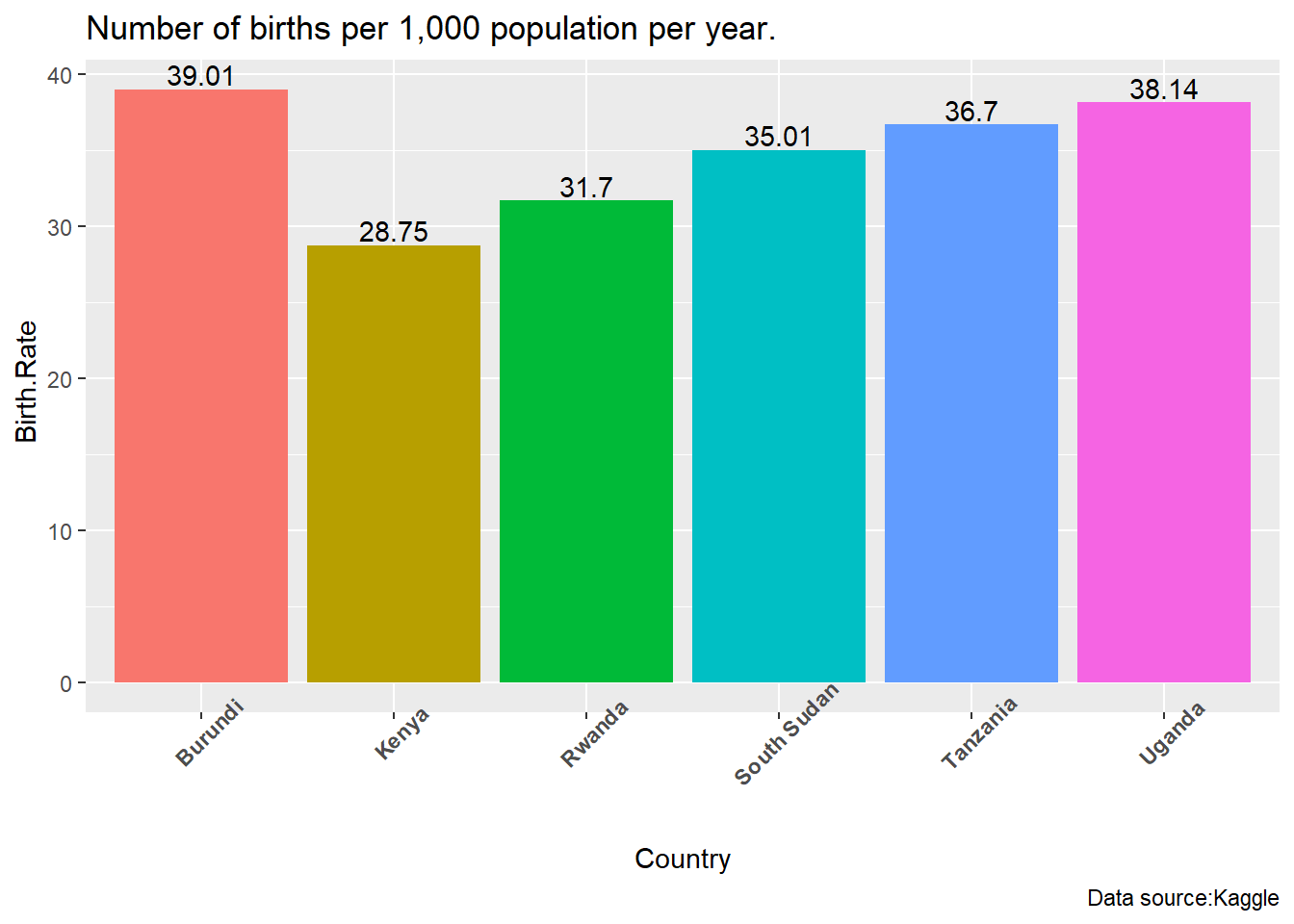

A higher birth rate generally contributes to population growth, while a lower birth rate may result in population decline or stabilization. It seems there is no much difference in the birth rate in all countries with the highest at 39 and the lowest at 29

CO2 Emissions

Code

east_africa %>% ggplot(aes(Country,as.numeric(gsub(",","", Co2.Emissions)), fill = Country, label = Co2.Emissions))+geom_col()+
  geom_text(vjust = -0.2)+
  labs(title = "Carbon dioxide emissions in tons.",
       y = "Co2.Emissions",
       caption = "Data source:Kaggle")+
  theme(axis.text.x = element_text(angle = 45, face = "bold"),legend.position = "none")+scale_y_continuous(labels = comma)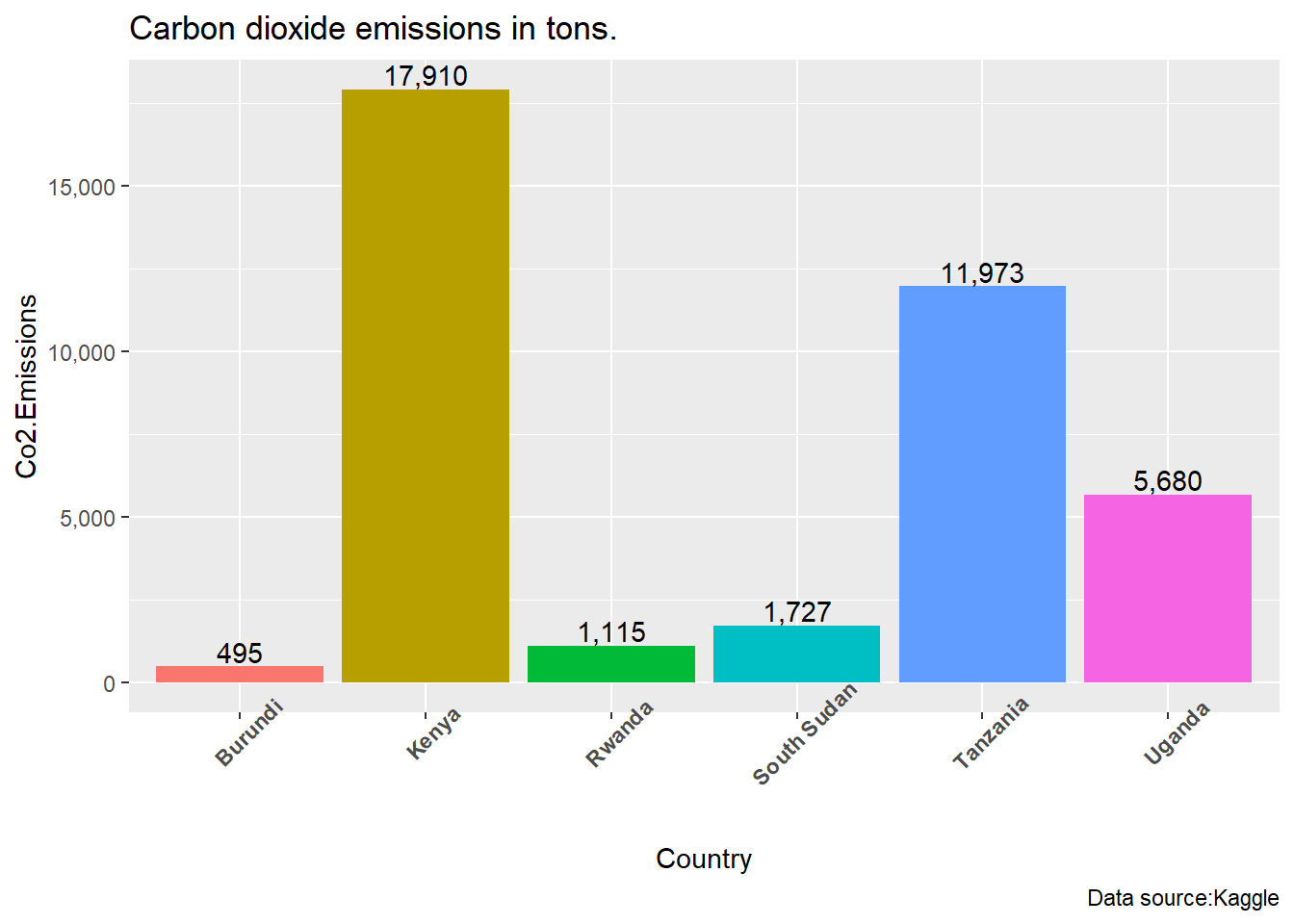

CO2 emissions refer to the release of carbon dioxide into the atmosphere, primarily as a result of human activities such as burning fossil fuels (coal, oil, and natural gas), industrial processes, deforestation, and certain agricultural practices.More developed countries are the greatter emission of CO2 in this case we have kenya leading and Burundi with the lowest.The increase in CO2 concentrations is a major driver of the observed rise in global temperatures, with cascading effects on weather patterns, sea levels, and ecosystems.The transition to cleaner energy sources, such as solar and wind power, is a key strategy to reduce CO2 emissions from the energy sector.

Forested Area (%)

Code

east_africa %>% ggplot(aes(Country,as.numeric(sub("%","",Forested.Area....)), fill = Country, label =  Forested.Area.... ))+geom_col()+
  geom_text(vjust = -0.2)+
  labs(title = "Percentage of land area covered by forests.",
       y =  "Forested.Area",
       caption = "Data source:Kaggle")+
  theme(axis.text.x = element_text(angle = 45, face = "bold"),legend.position = "none")

Warning: Removed 1 row containing missing values or values outside the scale range
(`geom_col()`).

Warning: Removed 1 row containing missing values or values outside the scale range
(`geom_text()`).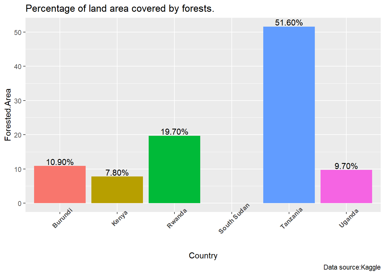

Forest area refers to the total land area covered by trees with varying degrees of density and canopy cover. Forests are crucial for maintaining ecological balance, supporting biodiversity, providing habitats for wildlife, and contributing to the overall health of the planet. They play a vital role in mitigating climate change by helping to regulate the global climate.Tanzania has the highest forest cover and Kenya has the lowest.

Gasoline_Price

Code

east_africa %>% ggplot(aes(Country,as.numeric(gsub("\\$","",Gasoline.Price)), fill = Country, label =  Gasoline.Price))+geom_col()+
  geom_text(vjust = -0.2)+
  labs(title = "Price of gasoline per liter in local currency.",
       y =  "Gasoline.Price",
       caption = "Data source:Kaggle")+
  theme(axis.text.x = element_text(angle = 45, face = "bold"),legend.position = "none")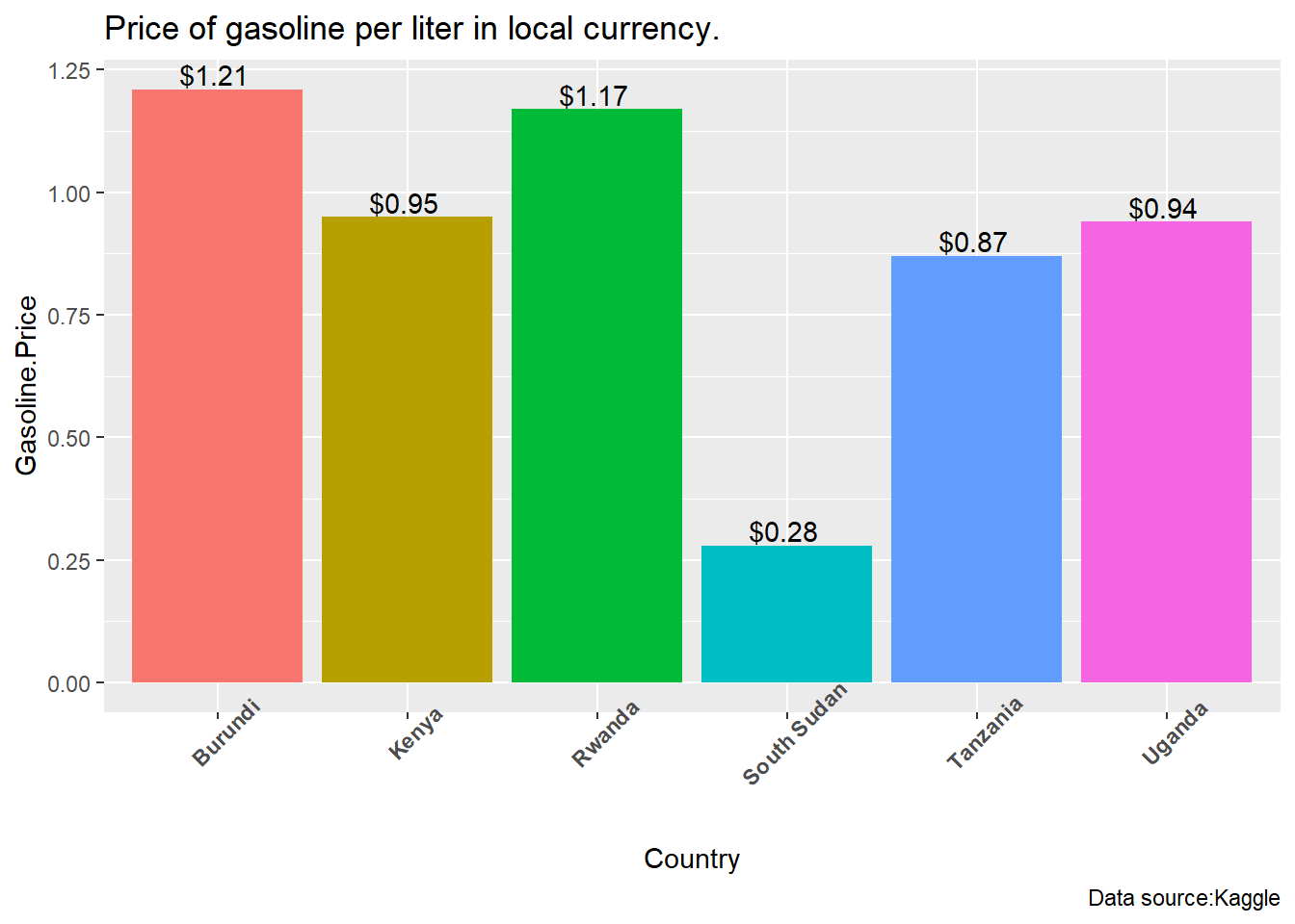

Difference in gasoline prices may be as a result of various factors including Exchange rates,taxes,government policies and subsidies,demand and supply,infrastructure and transportation costs and global oil prices.Gasoline prices plays a critical role on the cost of living, high gasoline prices can lead high cost of living

Life Expectancy

Code

east_africa %>% ggplot(aes(Country,Life.expectancy, fill = Country, label =  Life.expectancy))+geom_col()+
  geom_text(vjust = -0.2)+
  labs(title = "Average number of years a newborn is expected to live.",
       y =  "Life.expectancy",
       caption = "Data source:Kaggle")+
  theme(axis.text.x = element_text(angle = 45, face = "bold"),legend.position = "none")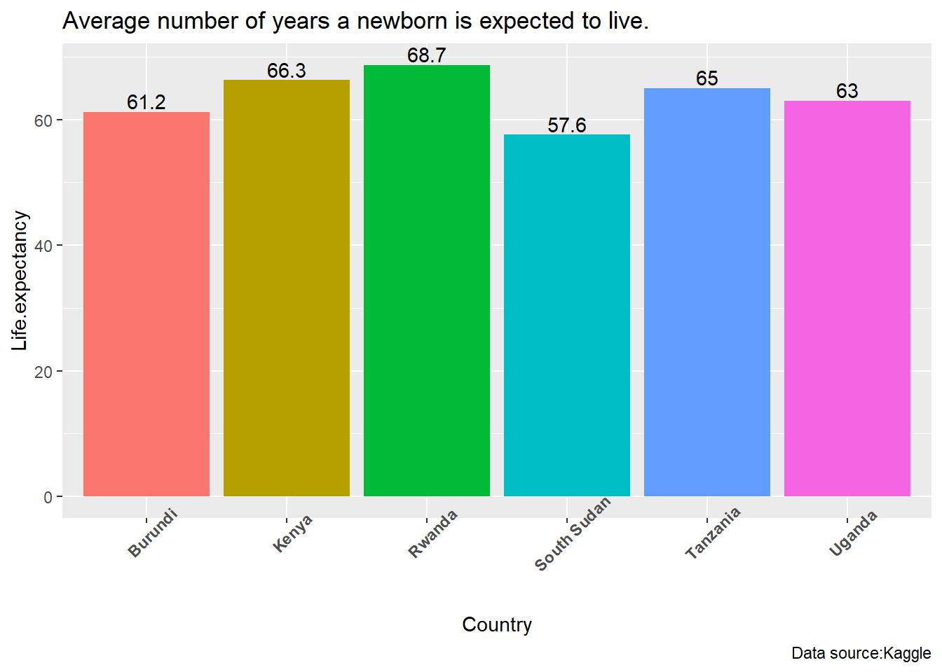

life expectancy is critical to asses the economy of a country.A population with a higher life expectancy generally means a larger working-age population. This can contribute to a larger labor force, which, if effectively utilized, can lead to increased productivity and economic output. most of the countries in East Africa has life expectancy greater than 60, with Rwanda leading at 69

Infant Mortality

Code

east_africa %>% ggplot(aes(Country,Infant.mortality , fill = Country, label =  Infant.mortality ))+geom_col()+
  geom_text(vjust = -0.1)+
  labs(title = "Number of deaths per 1,000 live births before reaching one year of age",
       y =  "Infant.mortality ",
       caption = "Data source:Kaggle")+
  theme(axis.text.x = element_text(angle = 45, face = "bold"),legend.position = "none")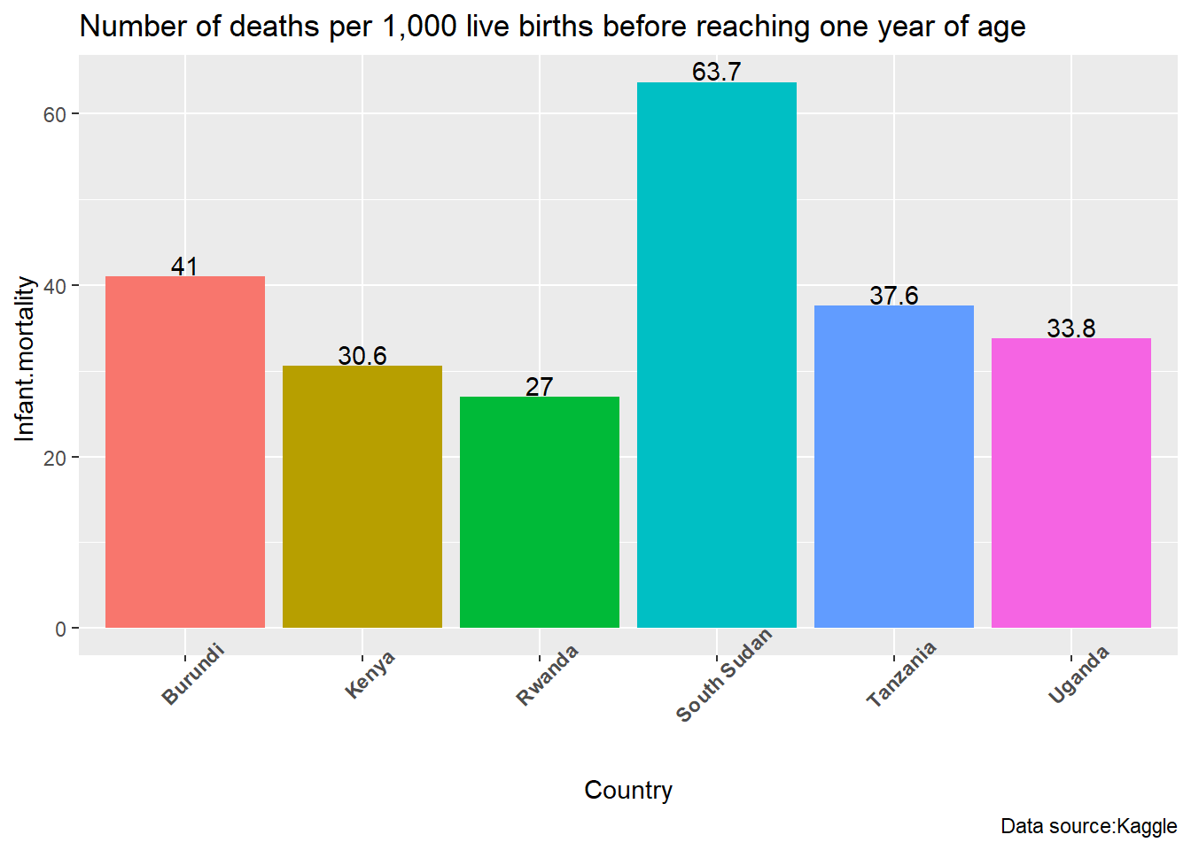

Infant mortality, defined as the death of a child before their first birthday, is an important indicator of a population’s health and the quality of healthcare services. It is usually expressed as the number of infant deaths per 1,000 live births. High infant mortality rates can be indicative of underlying health and socio-economic challenges Improving these factors can contribute to a reduction in infant mortality.Countrie with better health care report small cases e.g Rwanda, whereas those with poor access to health care and adverse socio economic condition have more cases.

Maternal Mortality Ratio

Code

east_africa %>% ggplot(aes(Country,Maternal.mortality.ratio  , fill = Country, label =  Maternal.mortality.ratio  ))+geom_col()+
  geom_text(vjust = -0.1)+
  labs(title = "Number of maternal deaths per 100,000 live births.",
       y =  "Maternal.mortality.ratio  ",
       caption = "Data source:Kaggle")+
  theme(axis.text.x = element_text(angle = 45, face = "bold"),legend.position = "none")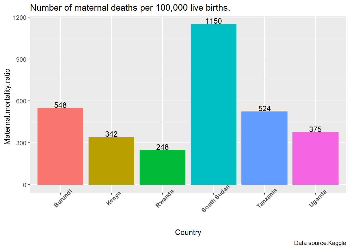

This ratio is a crucial indicator in assessing the health and well-being of pregnant individuals and reflects the quality of maternal healthcare services.Maternal mortality can result from a range of causes, including complications during pregnancy, childbirth, and the postpartum period. Common causes include hemorrhage, infections, hypertensive disorders, and unsafe abortions.South Sudan has the highest number while Rwanda has the lowest

Minimum Wage

Code

east_africa %>% ggplot(aes(Country,as.numeric(sub("\\$","", Minimum.wage))  , fill = Country, label =  Minimum.wage ))+geom_col()+
  geom_text(vjust = -0.1)+
  labs(title = " Minimum wage level in local currency.",
       y =  "Minimum.wage ",
       caption = "Data source:Kaggle")+
  theme(axis.text.x = element_text(angle = 45, face = "bold"),legend.position = "none")

Warning: Removed 3 rows containing missing values or values outside the scale range
(`geom_col()`).

Warning: Removed 3 rows containing missing values or values outside the scale range
(`geom_text()`).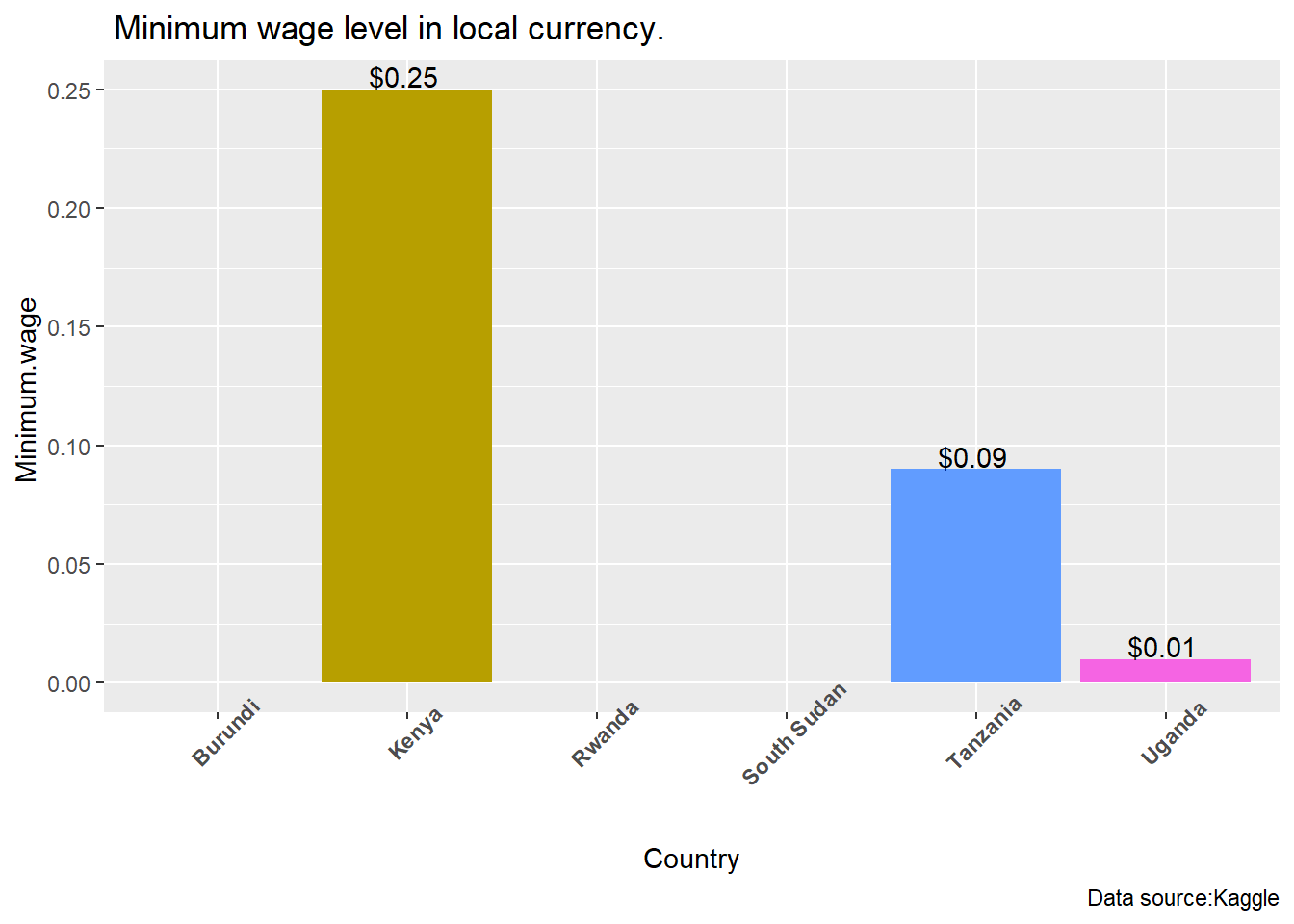

The minimum wage is the lowest amount of compensation that employers are legally required to pay their employees for their work. Minimum wage levels vary widely from country to country and often within regions or states of a country. These rates are typically established by law and are intended to provide a basic standard of living for workers. several factors can influence the determination of minimum wage levels, including the cost of living, inflation rates, economic conditions, and government policies.

Out of Pocket Health Expenditure

Code

east_africa %>% ggplot(aes(Country,as.numeric(gsub("%","", Out.of.pocket.health.expenditure))  , fill = Country, label =   Out.of.pocket.health.expenditure ))+geom_col()+
  geom_text(vjust = -0.1)+
  labs(title = " Percentage of total health expenditure paid out-of-pocket by individuals.",
       y =  " Out.of.pocket.health.expenditure",
       caption = "Data source:Kaggle")+
  theme(axis.text.x = element_text(angle = 45, face = "bold"),legend.position = "none")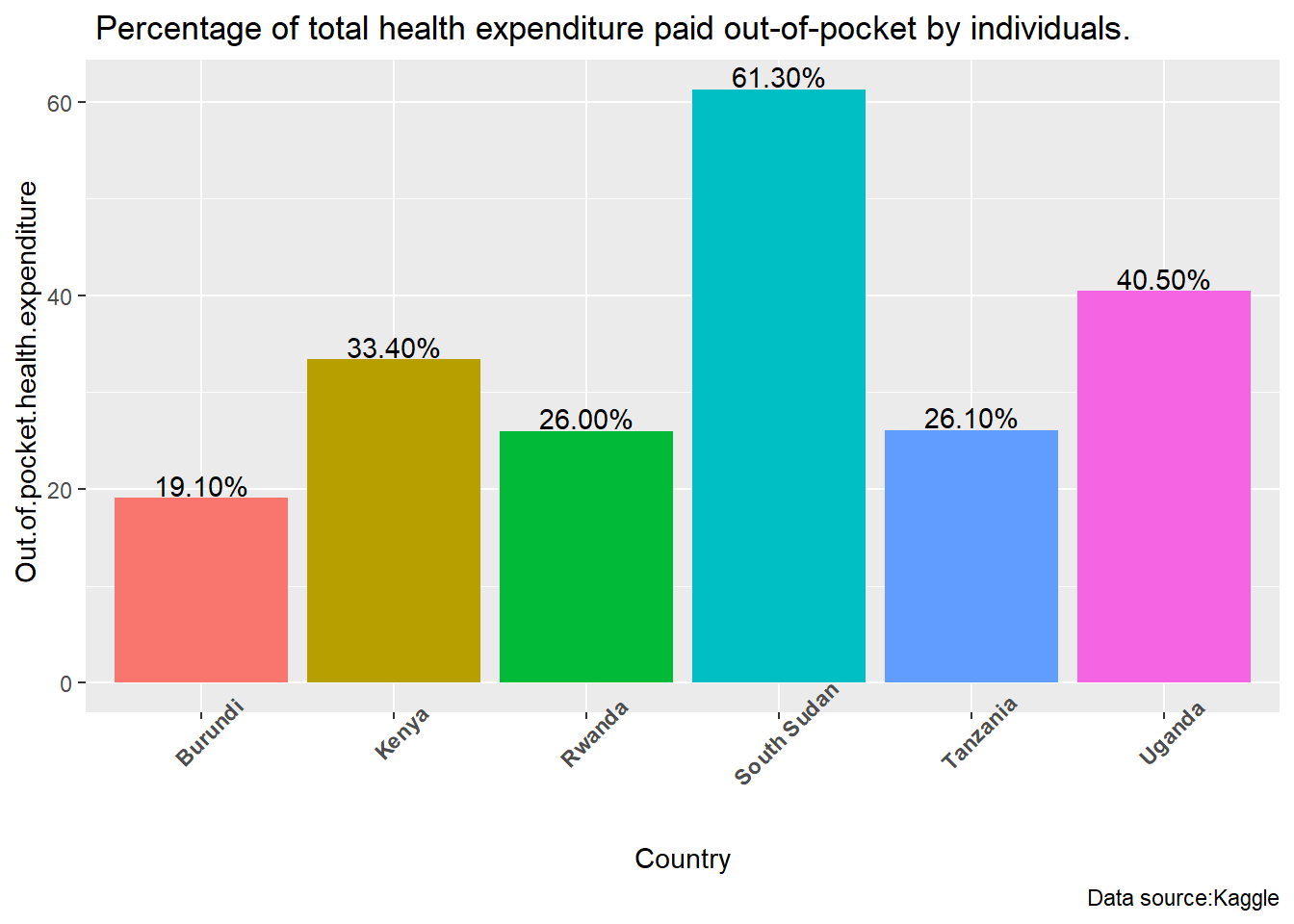

Out-of-pocket health expenditure refers to the direct payments made by individuals at the time they receive healthcare services. These payments are made by individuals to healthcare providers and can include expenses such as co-payments, deductibles, and payments for services that are not covered by health insurance. The extent of out-of-pocket health expenditure varies widely from country to country. In some countries, individuals may have comprehensive health coverage with minimal out-of-pocket expenses, while in others, individuals may bear a significant portion of their healthcare costs eg in our case South Sudan.

Population

Code

east_africa %>% ggplot(aes(Country,as.numeric(gsub(",","",  Population))  , fill = Country, label =    Population))+geom_col()+
  geom_text(vjust = -0.1)+
  labs(title = "Total population of the country.",
       y =  "  Population",
       caption = "Data source:Kaggle")+
  theme(axis.text.x = element_text(angle = 45, face = "bold"),legend.position = "none")+scale_y_continuous(label = comma)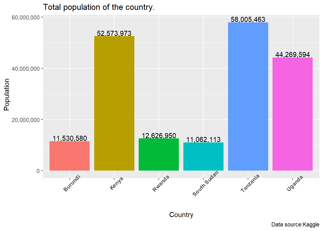

Population is directly related to total land area. Countries with huge land areas have large population

Labor Force Participation (%)

Code

east_africa %>% ggplot(aes(Country,as.numeric(gsub("%","", Population..Labor.force.participation....))  , fill = Country, label =   Population..Labor.force.participation....))+geom_col()+
  geom_text(vjust = -0.1)+
  labs(title = " Percentage of the population that is part of the labor force.",
       y =  " Labor.force.participation",
       caption = "Data source:Kaggle")+
  theme(axis.text.x = element_text(angle = 45, face = "bold"),legend.position = "none")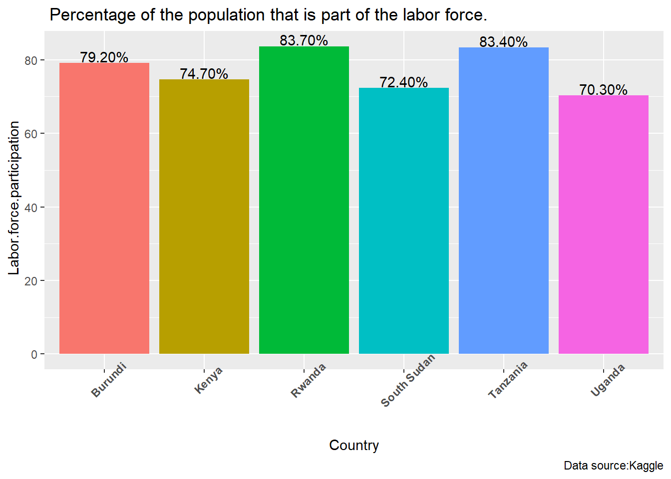

In many East African countries, agriculture is a significant contributor to employment. A large portion of the population is engaged in subsistence farming or agricultural-related activities. However, there is a growing recognition of the need for economic diversification to create more non-agricultural job opportunities.

Tax levenue % of GDP

Code

east_africa %>% ggplot(aes(Country,as.numeric(gsub("%","", Tax.revenue....))  , fill = Country, label =   Tax.revenue....))+geom_col()+
  geom_text(vjust = -0.1)+
  labs(title = " Tax revenue as a percentage of GDP.",
       y =  "Tax.revenue.",
       caption = "Data source:Kaggle")+
  theme(axis.text.x = element_text(angle = 45, face = "bold"),legend.position = "none")

Warning: Removed 1 row containing missing values or values outside the scale range
(`geom_col()`).

Warning: Removed 1 row containing missing values or values outside the scale range
(`geom_text()`).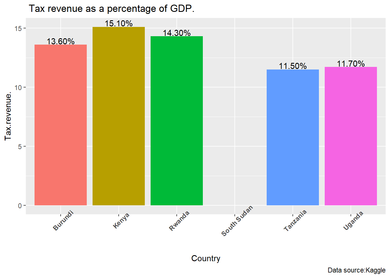

The tax-to-GDP ratio is a key economic indicator that measures the proportion of a country’s economic output (Gross Domestic Product, GDP) that is collected as taxes. This ratio provides insights into the overall tax burden on the economy and the extent to which the government relies on taxation to fund public expenditures. Countries with good taxing system are associated with greater ratio.Recommended ratio should be above 15%.

Total Tax Rate

Code

east_africa %>% ggplot(aes(Country,as.numeric(gsub("%","", Total.tax.rate))  , fill = Country, label =   Total.tax.rate))+geom_col()+
  geom_text(vjust = -0.1)+
  labs(title = "Overall tax burden as a percentage of commercial profits.",
       y =  "Total.tax.rate",
       caption = "Data source:Kaggle")+
  theme(axis.text.x = element_text(angle = 45, face = "bold"),legend.position = "none")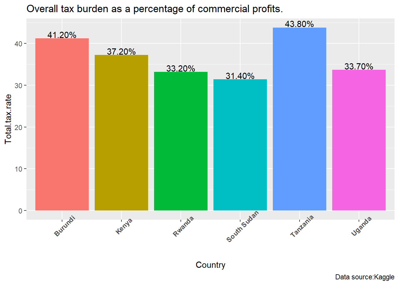

The total tax rate is a measure that reflects the total amount of taxes paid by a business as a percentage of its profits. It is commonly used to assess the overall tax burden on businesses and is a key indicator for understanding the tax environment in a particular country. The total tax rate includes not only corporate income taxes but also other taxes and contributions that businesses may be required to pay.This can influence the willingness of investor to invest in a particular country.

Unemployment Rate

Code

east_africa %>% ggplot(aes(Country,as.numeric(gsub("%","",  Unemployment.rate ))  , fill = Country, label = Unemployment.rate ))+geom_col()+
  geom_text(vjust = -0.1)+
  labs(title = " Percentage of the labor force that is unemployed.",
       y =  " Unemployment.rate ",
       caption = "Data source:Kaggle")+
  theme(axis.text.x = element_text(angle = 45, face = "bold"),legend.position = "none")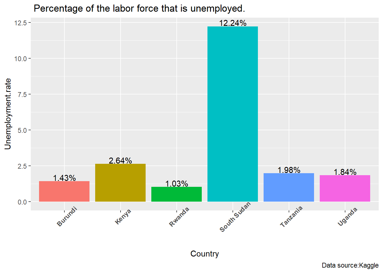

The unemployment rate is a key economic indicator that measures the percentage of the labor force that is unemployed and actively seeking employment. It provides insights into the health of the labor market and the overall economic conditions. South Sudan has the highest unemployment rate. This may be attributed to poor economic condition in the country.

Urban Population

Code

east_africa %>% ggplot(aes(Country,as.numeric(gsub(",","",  Urban_population ))  , fill = Country, label =Urban_population ))+geom_col()+
  geom_text(vjust = -0.2)+
  labs(title = "  Percentage of the population living in urban areas.",
       y =  " Urban population ",
       caption = "Data source:Kaggle")+
  theme(axis.text.x = element_text(angle = 45, face = "bold"),legend.position = "none")+scale_y_continuous(label = comma)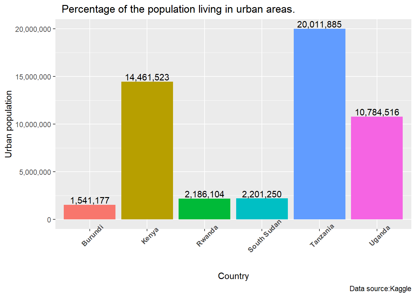

Urban population refers to the number of people residing in urban areas, which are characterized by a higher population density and infrastructure development compared to rural areas.Urbanization is influenced by various factors, including industrialization, economic opportunities in urban centers, improved infrastructure, better access to education and healthcare, and changes in lifestyle preferences.

Summary

The exploration of East African countries through comprehensive data analysis has unveiled a multifaceted view of the region. Covering a range of key variables such as population density, economic indicators, healthcare metrics, and more, the analysis has painted a vivid picture of the socio-economic landscapes of nations like Kenya, Tanzania, Uganda, Rwanda, Burundi, and South Sudan.

The dataset has allowed us to delve into diverse aspects, from the economic reliance on agriculture to the environmental impact reflected in CO2 emissions. We’ve observed variations in healthcare indicators, from life expectancy and infant mortality to maternal mortality ratios, shedding light on the health and well-being of the population.

Moreover, social and economic factors such as minimum wage, out-of-pocket health expenditure, labor force participation, and tax rates have been scrutinized, offering insights into the economic conditions and government policies across the East African region. Urbanization trends, unemployment rates, and armed forces’ sizes have also contributed to our understanding of the broader dynamics at play.

In conclusion, this exploration underscores the complexity and diversity within the East African region. The analysis has not only provided a snapshot of the current state of these countries but also laid the groundwork for informed cross-country comparisons. The interplay of demographic, economic, and environmental factors highlights the intricate challenges and opportunities that each nation faces.

As we navigate through the data, it becomes evident that a holistic approach is essential for policymakers and stakeholders to address the unique needs of each country. Whether it’s planning for sustainable urbanization, improving healthcare systems, or formulating economic policies, a nuanced understanding of the data is paramount.

This journey into East Africa’s data landscape serves as a starting point for deeper discussions, further research, and informed decision-making. It is an invitation to explore the rich tapestry of cultures, challenges, and potentials that define this region. As we conclude this analysis, the hope is that these insights contribute to a more comprehensive understanding of East Africa and its trajectory in the global landscape.

References

United Nations Development Programme (UNDP). (2020). Human Development Report 2020. Retrieved from http://hdr.undp.org/sites/default/files/hdr2020.pdf

World Bank. (2020). World Development Indicators. Retrieved from https://databank.worldbank.org/source/world-development-indicators

World Health Organization (WHO). (2020). Global Health Observatory data repository. Retrieved from https://www.who.int/data/gho

International Labour Organization (ILO). (2020). ILOSTAT database. Retrieved from https://ilostat.ilo.org/

Central Intelligence Agency (CIA). (2020). The World Factbook. Retrieved from https://www.cia.gov/the-world-factbook/

African Development Bank Group. (2020). African Economic Outlook. Retrieved from https://www.afdb.org/en/knowledge/publications/african-economic-outlook