Will Kenyan GDP Growth Reach 10% by 2030?
As Kenya marches forward into the future, the question of its economic trajectory looms large on the national agenda. With ambitious development goals outlined in the Vision 2030 agenda, the country aspires to achieve sustained and inclusive economic growth that uplifts the lives of its citizens. At the heart of this vision lies the GDP growth rate, a key indicator of economic health and prosperity. In recent years, Kenya has made significant strides in its economic journey, with notable achievements in sectors such as agriculture, manufacturing, and services. However, as the nation sets its sights on the next decade, the question arises: will Kenya achieve a GDP growth rate of 10 percent by 2030?
This blog seeks to explore this pressing question by delving into the realm of time series analysis. By leveraging historical GDP data and employing sophisticated forecasting techniques, I aim to unravel the trends, patterns, and potential future trajectories of Kenya’s economic growth.
Trend in Kenya GDP Growth Rate
1990s - Early 2000s
In the early 1990s, Kenya embarked on economic reforms aimed at liberalizing the economy and attracting foreign investment. However, the country faced challenges such as political instability and corruption, which hampered economic growth.Despite these challenges, the late 1990s saw a period of moderate GDP growth driven by sectors like agriculture, manufacturing, and services. Political reforms and improved governance in the late 1990s and early 2000s contributed to a more favorable investment climate, supporting economic expansion.
Mid-2000s - Pre-Financial Crisis (2005-2007)
The mid-2000s witnessed a period of relatively robust GDP growth, fueled by increased investment in infrastructure, telecommunications, and financial services. Government initiatives to promote private sector development and attract foreign direct investment (FDI) also supported economic expansion. Kenya’s economy benefited from favorable global conditions, including high commodity prices and strong demand for exports.
Global Financial Crisis (2008-2009)
The global financial crisis of 2008-2009 had a significant impact on Kenya’s economy, leading to a slowdown in GDP growth.Reduced demand for exports, declining remittances, and disruptions in global trade negatively affected key sectors like agriculture, tourism, and manufacturing. The crisis exposed vulnerabilities in Kenya’s financial sector and highlighted the importance of diversifying the economy and strengthening resilience to external shocks. The political instability that erupted in Kenya in 2007 and 2008, following disputed presidential elections, severely impacted the country’s GDP growth trajectory. Widespread violence and ethnic clashes paralyzed economic activities, disrupted supply chains, and caused significant damage to infrastructure and businesses.Investor confidence plummeted, leading to capital flight and a contraction in GDP growth
Post-Crisis Recovery (2010-2013)
Following the global financial crisis, Kenya experienced a period of recovery and resumed GDP growth, supported by government stimulus measures and renewed investor confidence. Infrastructure development projects, such as the construction of roads, ports, and energy facilities, played a crucial role in driving economic activity and creating employment opportunities. Kenya’s vibrant services sector, including telecommunications, banking, and information technology, emerged as a key driver of growth during this period.
2010s - Recent Years (2014-2023):
The 2010s saw mixed economic performance, with periods of strong growth interspersed with slowdowns and challenges. Factors such as political uncertainty, security concerns, and adverse weather conditions (e.g., droughts) posed headwinds to economic expansion.Nevertheless, Kenya continued to attract investment in sectors like real estate, energy, and infrastructure, supported by government initiatives to improve the business environment and promote entrepreneurship.
Code
p2 <- data %>%
  ggplot(aes(year, gdp_growth)) +
  geom_line(aes(color = "Economic Growth"), linewidth = 1, linetype = 1) +
  geom_smooth(aes(color = "Trend Line"), method = "lm", se = FALSE, linetype = 1, show.legend = TRUE) +
  ylim(-2, 10) + xlim(1990, 2027) + theme_bw() +
  labs(caption = "Source of the Data: Central Bank of Kenya",
       y = "GDP Growth Rate(%)",
       x = "Year") +
  theme(plot.title = element_text(colour = "black", size = 15, face = "bold"),
        axis.text.x = element_text(colour = "black"),
        axis.text.y = element_text(color = "black"),
        axis.title.x = element_text(face = "bold"),
        axis.title.y = element_text(face = "bold"),
        legend.position = "bottom", legend.title =element_blank()) +
  scale_color_manual(values = c("Economic Growth" = "blue", "Trend Line" = "red"),
                     labels = c("Economic Growth", "Trend Line"))
p2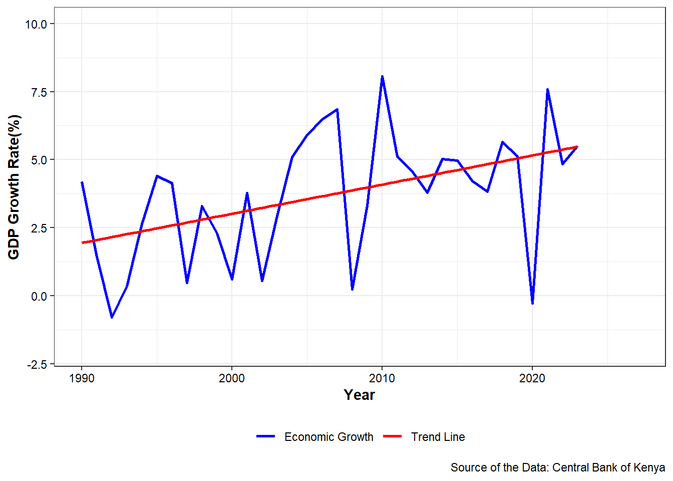
Using Holt-Winters Method for GDP Growth Rate Forecasting
To forecast Kenya’s GDP growth rate up to 2030, I chose the Holt-Winters method, a powerful and flexible time series forecasting technique. The Holt-Winters method, also known as the Exponential Smoothing State Space Model (ETS), is adept at capturing complex patterns in data, including level and trend components.
Why Holt-Winters?
Trend Detection: Our GDP growth rate data shows a clear trend over time, which is crucial for making accurate forecasts. The Holt-Winters method effectively captures and extrapolates this trend.
Flexibility: This method can be adapted to data with or without seasonal patterns. Since our GDP data lacks seasonality but exhibits a trend, we can disable the seasonal component (gamma) and still leverage the method’s strengths.
Simplicity and Interpretability: The Holt-Winters method is straightforward to implement and interpret, making it easier to explain the forecast results and underlying assumptions.
Proven Robustness: Widely used in economic forecasting, the Holt-Winters method is known for its robustness and reliability across various types of time series data.
Model Fitting and Forecasting
By fitting the Holt-Winters model to our historical GDP growth rate data and forecasting future values, we aim to provide reliable projections that inform economic planning and policy-making. The model captures the underlying trend, allowing us to make informed predictions about Kenya’s economic growth trajectory up to 2030.
Code
Holt-Winters exponential smoothing with trend and without seasonal component.

Call:
HoltWinters(x = gdp_ts, gamma = F)

Smoothing parameters:
 alpha: 0.5807826
 beta : 0.2718869
 gamma: FALSE

Coefficients:
       [,1]
a 5.3704952
b 0.2467251
Practical Interpretation Level (a = 5.3704952): The current GDP growth rate is around 5.37%. This is the baseline value from which future growth is projected.
Trend (b = 0.2467251): The GDP growth rate is projected to increase by approximately 0.25% per year. This indicates a positive growth trend in the GDP growth rate.
Why These Parameters Matter
Alpha = 0.5807826: The relatively high alpha value means the model is responsive to recent changes in GDP growth rate, allowing it to quickly adapt to new data.
Beta = 0.2718869: The moderate beta value indicates a stable trend estimation. The trend component is updated cautiously, which prevents overreacting to short-term fluctuations.
Gamma = FALSE: By setting gamma to FALSE, the model focuses solely on capturing the trend and level, which suits the nature of your data (no seasonality).
Prediction
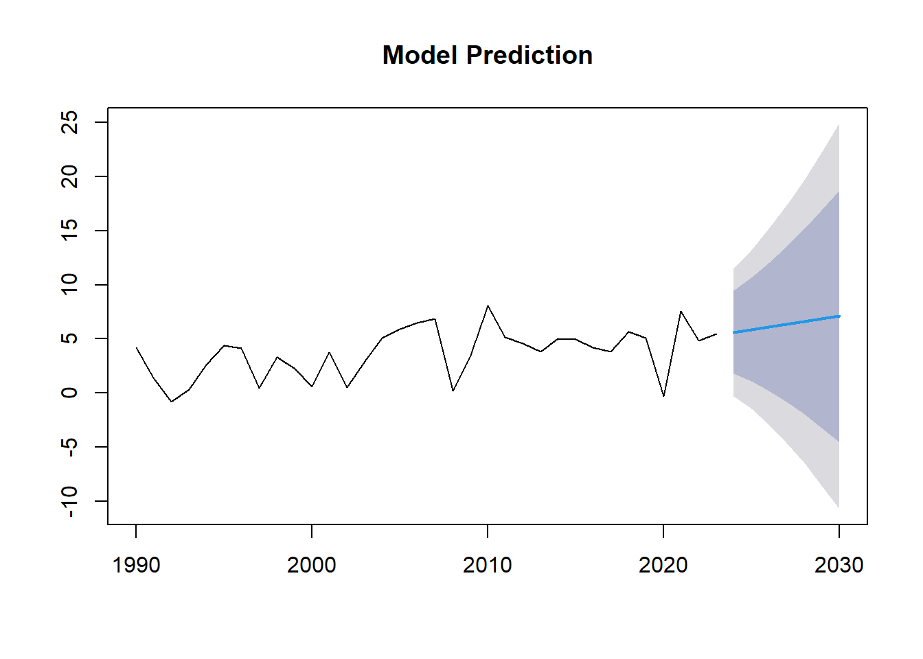
2024: The estimated GDP growth rate for 2024 is 5.62%.
2025:
The estimated GDP growth rate for 2025 is 5.86%.
2026:
The estimated GDP growth rate for 2026 is 6.11%.
2027:
The estimated GDP growth rate for 2027 is 6.36%.
2028:
The estimated GDP growth rate for 2028 is 6.60%.
2029:
The estimated GDP growth rate for 2029 is 6.85%.
2030:
The estimated GDP growth rate for 2030 is 7.10%.
Limitation of the Model
While the Holt-Winters method is a powerful tool for time series forecasting, it’s important to acknowledge its limitations:
Assumption of Stationarity: The Holt-Winters method assumes that the time series data is stationary, meaning that its statistical properties such as mean and variance do not change over time. In reality, economic data like GDP growth rates often exhibit non-stationarity due to various factors such as economic cycles, policy changes, and external shocks.
Limited Incorporation of External Factors: The model primarily relies on historical data to make forecasts and may not adequately capture the impact of external factors such as geopolitical events, changes in government policies, or technological advancements. These factors can significantly influence economic trends but are not explicitly accounted for in the Holt-Winters framework.
Sensitivity to Initial Conditions: The accuracy of forecasts produced by the Holt-Winters method can be sensitive to the initial values of the smoothing parameters (alpha, beta, and gamma). Choosing inappropriate initial values may result in suboptimal forecasts, especially for longer-term projections.
Inability to Handle Sudden Changes: The Holt-Winters method may struggle to adapt to sudden and unexpected changes in the data, such as economic recessions or financial crises. Since it relies heavily on past observations, it may take time for the model to adjust to new trends or patterns, leading to delayed or inaccurate forecasts during periods of volatility.
Difficulty in Interpreting Seasonality: While the Holt-Winters method can accommodate seasonal patterns in the data, interpreting and modeling seasonality accurately can be challenging, especially for longer time series with irregular or non-traditional seasonal patterns.
Risk of Overfitting: Like any forecasting model, there is a risk of overfitting the data, especially if the model is too complex or if there is noise in the data. Overfitting occurs when the model captures random fluctuations or noise in the data rather than underlying patterns, leading to poor performance on new, unseen data.
Limited Forecast Horizon: Forecast accuracy tends to decrease as the forecast horizon extends further into the future. This is because the uncertainty associated with longer-term forecasts increases, and the model may not capture complex dynamics or structural changes that occur over longer time periods.
Homogeneous Treatment of Data: The Holt-Winters method treats all data points equally in terms of their contribution to the forecast, which may not always be appropriate, especially if there are outliers or anomalies in the data that need to be weighted differently.
Acknowledging these limitations is essential for ensuring the appropriate application and interpretation of the Holt-Winters method in forecasting GDP growth rates or any other time series data. It’s often beneficial to complement the Holt-Winters method with other forecasting techniques and incorporate domain knowledge to enhance the robustness of forecasts.
Conclusion
In conclusion, our analysis utilizing the Holt-Winters exponential smoothing method provides valuable insights into the projected trajectory of Kenya’s GDP growth rate up to 2030. The forecasted GDP growth rates demonstrate a positive trend, with estimates increasing steadily from 5.62% in 2024 to 7.10% in 2030, based on the point forecasts. However, it’s crucial to interpret these forecasts within the context of the accompanying confidence intervals, which indicate the level of uncertainty surrounding the projections.