Multiple Linear Regression

Introduction

While simple linear regression models the relationship between two variables, multiple linear regression extends this concept to include multiple independent variables.

Assumptions of Multiple Linear Regression

Similar to simple linear regression, multiple linear regression relies on several assumptions:

• Linearity: The relationship between the dependent and independentvariables is linear.

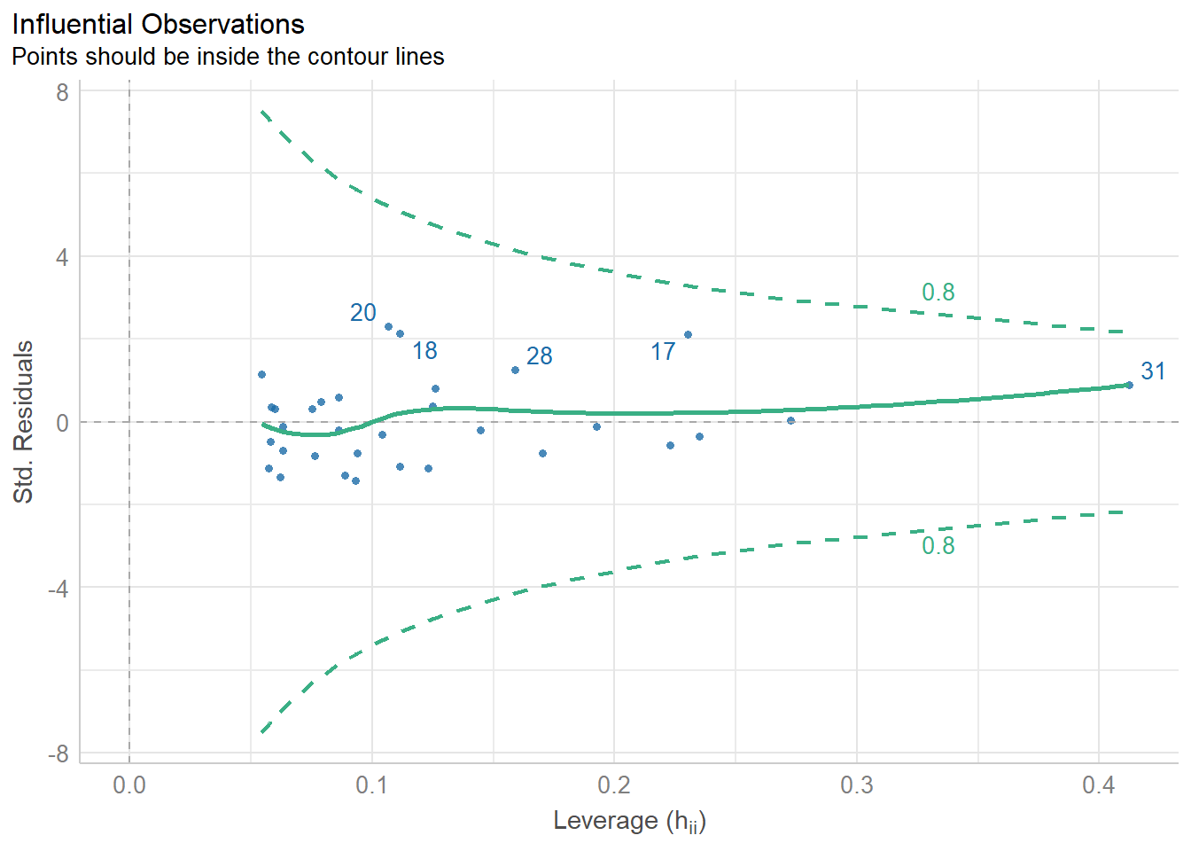
• Independence: The observations are independent of each other.

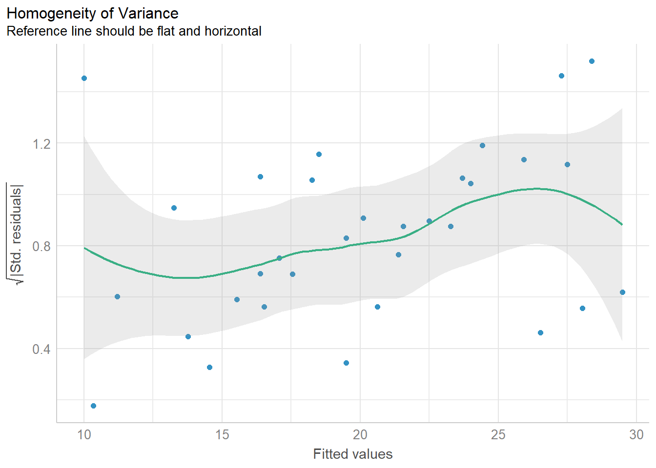
• Homoscedasticity: The variance of the residuals is constant across all levels of the independent variables.

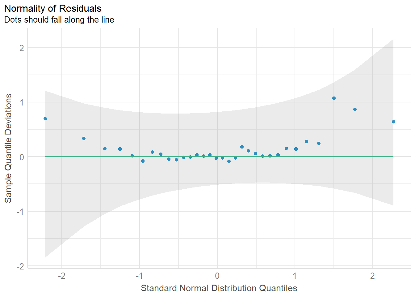
• Normality: The residuals are normally distributed.

Applications of Multiple Linear Regression

Multiple linear regressionfinds applications across various domains,including:

• Economics: Modeling the impact of multiple factors on GDP growth.

• Marketing: Predicting sales based on advertising spend, pricing, and promotional activities.

• Healthcare: Analyzing the effect of multiple treatments on patient outcomes.

• Environmental Science: Understanding the relationship between air quality and various pollutants.

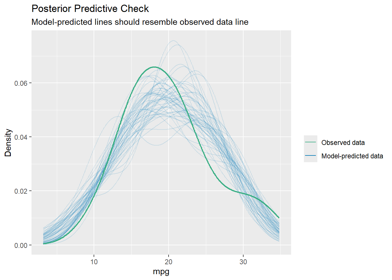
Performing Multiple Linear Regression in R Let’s walk through an example of performing multiple linear regression in R using mtcars dataset to determie the factors that affects fuel efficiency of cars

Sample Data

Code

head(mtcars)

                   mpg cyl disp  hp drat    wt  qsec vs am gear carb
Mazda RX4         21.0   6  160 110 3.90 2.620 16.46  0  1    4    4
Mazda RX4 Wag     21.0   6  160 110 3.90 2.875 17.02  0  1    4    4
Datsun 710        22.8   4  108  93 3.85 2.320 18.61  1  1    4    1
Hornet 4 Drive    21.4   6  258 110 3.08 3.215 19.44  1  0    3    1
Hornet Sportabout 18.7   8  360 175 3.15 3.440 17.02  0  0    3    2
Valiant           18.1   6  225 105 2.76 3.460 20.22  1  0    3    1

Code

mtcars$am <- factor(mtcars$am, labels = c("automatic", "manual"))

Fitting the Model using 3 variables

Code

fuel <- lm(mpg ~ wt+hp+am, data = mtcars)

Checking the Model Assumptions

• Normality

Code

library(performance)
check_normality(fuel)

OK: residuals appear as normally distributed (p = 0.071).

Code

plot(check_normality(fuel))

• Multicollinearity

Code

plot(check_collinearity(fuel))

Variable `Component` is not in your data frame :/

• Outliers

Code

plot(check_outliers(fuel))

• Homoscedasticity

Code

plot(check_heteroscedasticity(fuel))

• Autocorrelation

Code

check_autocorrelation(fuel)

Warning: Autocorrelated residuals detected (p = 0.044).

• Posterior predictive checks

Code

plot(check_posterior_predictions(fuel))

model-predicted lines seems not resembling well with the observed data lines

Interpretation of the model

Code

sjPlot::tab_model(fuel, show.intercept = F,show.reflvl = TRUE)

	mpg
Predictors	Estimates	CI	p
automatic	Reference
manual	2.08	-0.74 – 4.90	0.141
hp	-0.04	-0.06 – -0.02	0.001
wt	-2.88	-4.73 – -1.02	0.004
Observations	32
R2 / R2 adjusted	0.840 / 0.823

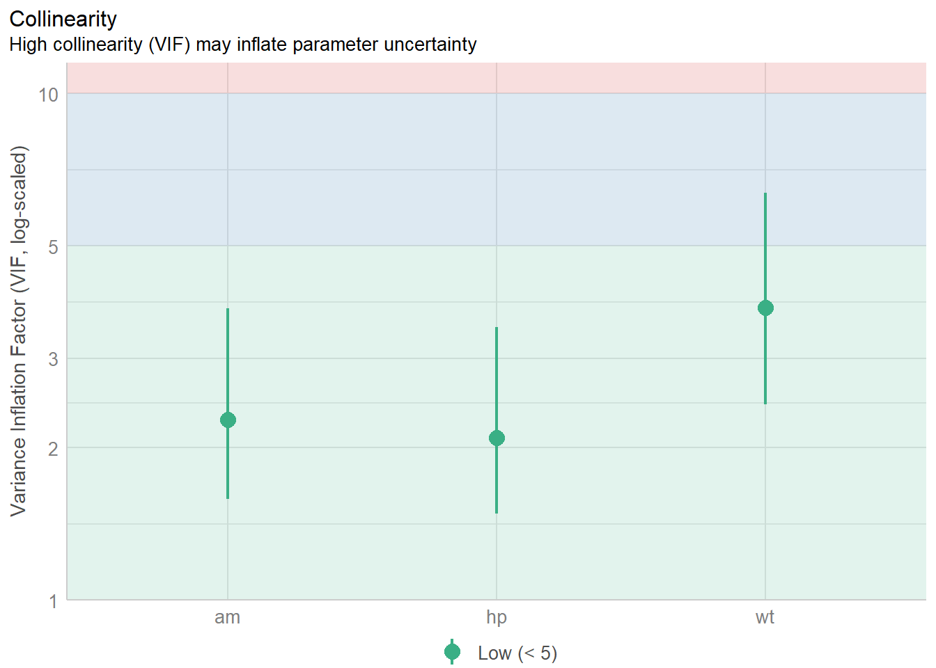
There is no significant difference in fuel efficiency between automatic and manual cars (p-value > 0.05). A one-unit increase in Gross horsepower (hp) increases fuel efficiency by 0.04 units on average, holding other factors constant. A one-unit increase in the weight of the car (wt) decreases fuel efficiency by 2.88 units of mpg on average, holding other factors constant. The adjusted R2 value of 82.3% indicates that the model explains 82.3% of the variation in the dependent variable (mpg), suggesting a good fit.

Conclusion

Multiple linear regression is a valuable tool for analyzing the relationship between a dependent variable and multiple independent variables. By checking model assumptions and interpreting the results accurately, we can make informed decisions based on the model’s findings. This blog post demonstrated how to perform multiple linear regression in R, interpret the results, and ensure the validity of the analysis through various diagnostic checks.