Simple Linear Regression

Introduction

Simple linear regression is a statistical method used to model the relationship between two continuous variables. It aims to describe how one variable (dependent variable,Y) changes in response to changes in another variable (independent variable,X).

Assumptions

• Linearity: The relationship between the independent and dependent variables is linear. This means that the change in the dependent variable is proportional to the change in the independent variable.

• Independence: The residuals (errors) are independent.

• Homoscedasticity: The residuals have constant variance at every level of X, ensuring that the variability in the response variable is consistent across values of the predictor variable.

• Normality: The residuals are normally distributed, which is important for making valid inferences.

• No outliers: Outliers can have a disproportionate effect on the regression model, leading to misleading results.

Applications of Simple Linear Regression

Simple linear regression is used in various domains, including:

• Economics: To model the relationship between income and expenditure.

• Healthcare: To predict patient outcomes based on treatment dosage.

• Marketing: To understand the impact of advertising spend on sales.

• Social Sciences: To analyze the relationship between education level and job satisfaction.

Performing Simple Linear Regression in R

Let’s walk through a simple example of performing linear regression in R. We’ll use a dataset that includes the advertising expenditure (in thousands of dollars) and the corresponding sales (in thousands of units).

Load the Data

Code

# Sample data
advertising_data <- data.frame(
  ad_spend = c(2.3, 3.5, 5.0, 7.2, 8.5, 10.0, 12.5, 15.0, 17.5, 20.0),
  sales = c(4.5, 5.1, 7.0, 8.8, 10.2, 11.5, 14.0, 15.5, 17.0, 19.0)
)

Plot the Data

Code

# Plotting the data
library(tidyverse)
advertising_data %>% 
  ggplot(aes(ad_spend,sales))+geom_point()+geom_smooth(method = lm,se = FALSE)+labs(title = "Sales vs. Advertising Spend",
                                                                                    x = "Advertising Spend (in thousands of dollars)",
                                                                                    y = "Sales (in thousands of units)")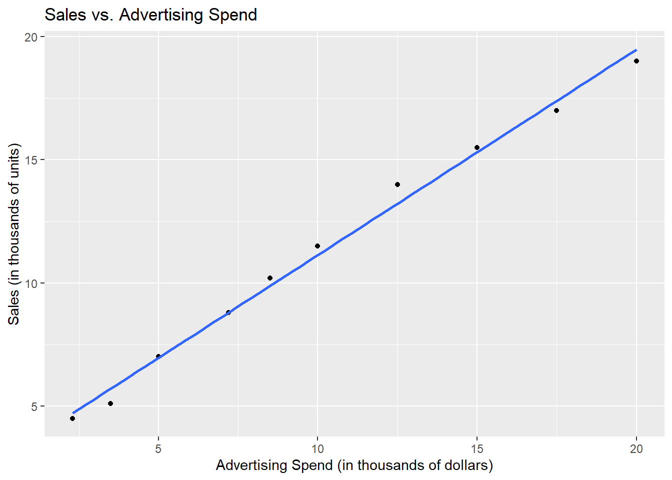

fitting the model

Code

# Fitting the linear model
model <- lm(sales ~ ad_spend, data=advertising_data)

# Display the model summary
sjPlot::tab_model(model)

	sales
Predictors	Estimates	CI	p
(Intercept)	2.79	2.10 – 3.47	<0.001
ad spend	0.83	0.78 – 0.89	<0.001
Observations	10
R2 / R2 adjusted	0.993 / 0.992

Model Assuptions

• Normality

Code

library(performance)
check_normality(model)

OK: residuals appear as normally distributed (p = 0.837).

• Outliers

Code

check_outliers(model)

OK: No outliers detected.
- Based on the following method and threshold: cook (0.8).
- For variable: (Whole model)

• Homoscedasticity

Code

check_heteroscedasticity(model)

OK: Error variance appears to be homoscedastic (p = 0.634).

Interpretation

The coefficient of the independent variable (ad_spend) in the model summary indicates that for every one thousand dollar increase in advertising spending, sales increase by 830 dollars on average, holding all other factors constant. This relationship is statistically significant at the 95% confidence level.

The R2 value of 0.993 suggests that 99.3% of the variation in sales can be explained by the variation in advertising spending. This high R2 value indicates a very good fit of the model to the data.

Conclusion

Simple linear regression is a powerful tool for understanding the relationship between two continuous variables and making predictions. By ensuring the assumptions of the model are met, we can make reliable inferences from the data. This blog post demonstrated how to perform simple linear regression in R, interpret the results, and check model assumptions to ensure the validity of the analysis.