Decision Trees in R

Introduction

Decision trees are a popular and intuitive method for both classification and regression tasks in machine learning. They work by splitting the data into subsets based on the value of input features, making a sequence of decisions that lead to a prediction. R provides powerful packages such as rpart and caret to easily build and visualize decision trees.

Key Steps in Building a Decision Tree in R

Data Preparation: Cleaning and preparing data for analysis.

Model Training: Building the decision tree model.

Model Evaluation: Assessing the model’s performance.

Model Visualization: Visualizing the decision tree.

Prediction: Using the trained model to make predictions on new data.

Example: Predicting Species with Decision Trees

Let’s walk through an example using a decision tree model to classify species in the iris dataset.

Load Necessary Packages r

Code

# install.packages("rpart")
# install.packages("rpart.plot")
# install.packages("caret")
# install.packages("e1071") # For support vector machines

library(rpart)
library(rpart.plot)
library(caret)
library(e1071)

Load and Prepare the Data

We’ll use the built-in iris dataset to predict the species of iris flowers based on their features.

Code

# Load the data
data <- iris

# Split the data into training and testing sets
set.seed(123)
train_index <- createDataPartition(data$Species, p = 0.8, list = FALSE)
train_data <- data[train_index, ]
test_data <- data[-train_index, ]

Train the Decision Tree Model

We’ll use the rpart function to train the decision tree model.

Code

# Train the model
model <- rpart(Species ~ ., data = train_data, method = "class")

# View the model summary
print(model)

n= 120 

node), split, n, loss, yval, (yprob)
      * denotes terminal node

1) root 120 80 setosa (0.33333333 0.33333333 0.33333333)  
  2) Petal.Length< 2.45 40  0 setosa (1.00000000 0.00000000 0.00000000) *
  3) Petal.Length>=2.45 80 40 versicolor (0.00000000 0.50000000 0.50000000)  
    6) Petal.Width< 1.75 42  3 versicolor (0.00000000 0.92857143 0.07142857) *
    7) Petal.Width>=1.75 38  1 virginica (0.00000000 0.02631579 0.97368421) *

Visualize the Decision Tree

Use the rpart.plot package to visualize the decision tree.

Code

# Visualize the decision tree
rpart.plot(model)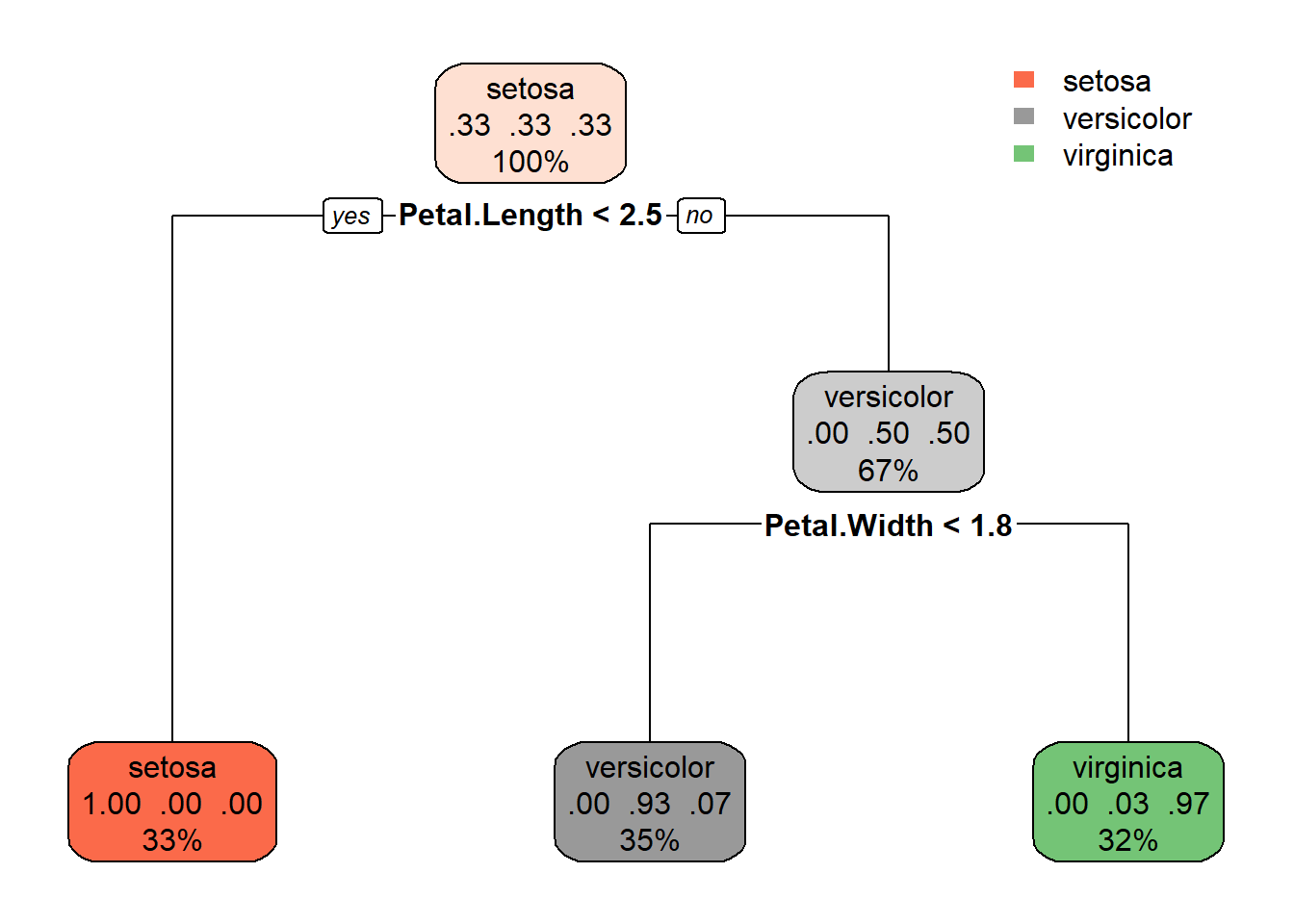

Evaluate the Model

Assess the model’s performance on the testing set.

Code

# Make predictions on the testing set
predictions <- predict(model, newdata = test_data, type = "class")

# Create a confusion matrix
conf_matrix <- confusionMatrix(predictions, test_data$Species)
print(conf_matrix)

Confusion Matrix and Statistics

            Reference
Prediction   setosa versicolor virginica
  setosa         10          0         0
  versicolor      0         10         2
  virginica       0          0         8

Overall Statistics
                                          
               Accuracy : 0.9333          
                 95% CI : (0.7793, 0.9918)
    No Information Rate : 0.3333          
    P-Value [Acc > NIR] : 8.747e-12       
                                          
                  Kappa : 0.9             
                                          
 Mcnemar's Test P-Value : NA              

Statistics by Class:

                     Class: setosa Class: versicolor Class: virginica
Sensitivity                 1.0000            1.0000           0.8000
Specificity                 1.0000            0.9000           1.0000
Pos Pred Value              1.0000            0.8333           1.0000
Neg Pred Value              1.0000            1.0000           0.9091
Prevalence                  0.3333            0.3333           0.3333
Detection Rate              0.3333            0.3333           0.2667
Detection Prevalence        0.3333            0.4000           0.2667
Balanced Accuracy           1.0000            0.9500           0.9000

Prediction on New Data

Use the trained model to make predictions on new data.

Code

# New data for prediction
new_data <- data.frame(
  Sepal.Length = c(5.1, 6.5),
  Sepal.Width = c(3.5, 3.0),
  Petal.Length = c(1.4, 5.2),
  Petal.Width = c(0.2, 2.0)
)

# Predict species for new data
new_predictions <- predict(model, newdata = new_data, type = "class")
new_predictions

        1         2 
   setosa virginica 
Levels: setosa versicolor virginica