Random Forest

Introduction

Random Forest is a powerful ensemble learning method used for classification and regression tasks. It operates by constructing multiple decision trees during training and outputting the mode of the classes (classification) or mean prediction (regression) of the individual trees. This method improves the model’s accuracy and reduces overfitting. R provides excellent packages such as randomForest and caret to build and evaluate random forests.

Key Steps in Building a Random Forest in R

Data Preparation: Cleaning and preparing data for analysis.

Model Training: Building the random forest model.

Model Evaluation: Assessing the model’s performance.

Prediction: Using the trained model to make predictions on new data.

Example: Predicting Species with Random Forest

Let’s walk through an example using a random forest model to classify species in the iris dataset.

Install and Load Necessary Packages

r

Code

# install.packages("randomForest")
# install.packages("caret")

library(randomForest)
library(caret)

Load and Prepare the Data

Code

# Load the data
data <- iris

# Split the data into training and testing sets
set.seed(123)
train_index <- createDataPartition(data$Species, p = 0.8, list = FALSE)
train_data <- data[train_index, ]
test_data <- data[-train_index, ]

Train the Random Forest Model

Code

# Train the model
model <- train(Species ~ ., data = train_data,
               method = "rf",
               importance = TRUE)

# View the model summary
print(model)

Random Forest 

120 samples
  4 predictor
  3 classes: 'setosa', 'versicolor', 'virginica' 

No pre-processing
Resampling: Bootstrapped (25 reps) 
Summary of sample sizes: 120, 120, 120, 120, 120, 120, ... 
Resampling results across tuning parameters:

  mtry  Accuracy   Kappa    
  2     0.9475159  0.9203020
  3     0.9455403  0.9172896
  4     0.9471579  0.9197251

Accuracy was used to select the optimal model using the largest value.
The final value used for the model was mtry = 2.

Evaluate the Model

Assess the model’s performance on the testing set.

Code

# Make predictions on the testing set
predictions <- predict(model, newdata = test_data)

# Create a confusion matrix
conf_matrix <- confusionMatrix(predictions, test_data$Species)
print(conf_matrix)

Confusion Matrix and Statistics

            Reference
Prediction   setosa versicolor virginica
  setosa         10          0         0
  versicolor      0         10         2
  virginica       0          0         8

Overall Statistics
                                          
               Accuracy : 0.9333          
                 95% CI : (0.7793, 0.9918)
    No Information Rate : 0.3333          
    P-Value [Acc > NIR] : 8.747e-12       
                                          
                  Kappa : 0.9             
                                          
 Mcnemar's Test P-Value : NA              

Statistics by Class:

                     Class: setosa Class: versicolor Class: virginica
Sensitivity                 1.0000            1.0000           0.8000
Specificity                 1.0000            0.9000           1.0000
Pos Pred Value              1.0000            0.8333           1.0000
Neg Pred Value              1.0000            1.0000           0.9091
Prevalence                  0.3333            0.3333           0.3333
Detection Rate              0.3333            0.3333           0.2667
Detection Prevalence        0.3333            0.4000           0.2667
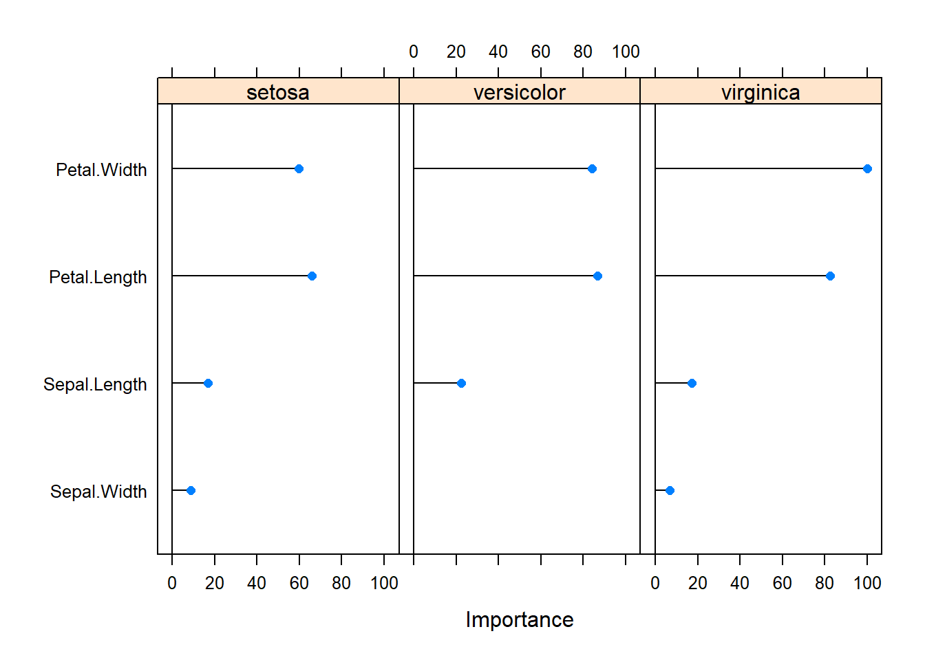
Balanced Accuracy           1.0000            0.9500           0.9000

Feature Importance

Examine the importance of each feature in the model.

Code

# View feature importance
plot(varImp(model))

Prediction on New Data

Use the trained model to make predictions on new data.

Code

# New data for prediction
new_data <- data.frame(
  Sepal.Length = c(5.1, 6.5),
  Sepal.Width = c(3.5, 3.0),
  Petal.Length = c(1.4, 5.2),
  Petal.Width = c(0.2, 2.0)
)

# Predict species for new data
new_predictions <- predict(model, newdata = new_data)
new_predictions

[1] setosa    virginica
Levels: setosa versicolor virginica

predicted new data

Code

new_data$Species <- new_predictions
new_data

  Sepal.Length Sepal.Width Petal.Length Petal.Width   Species
1          5.1         3.5          1.4         0.2    setosa
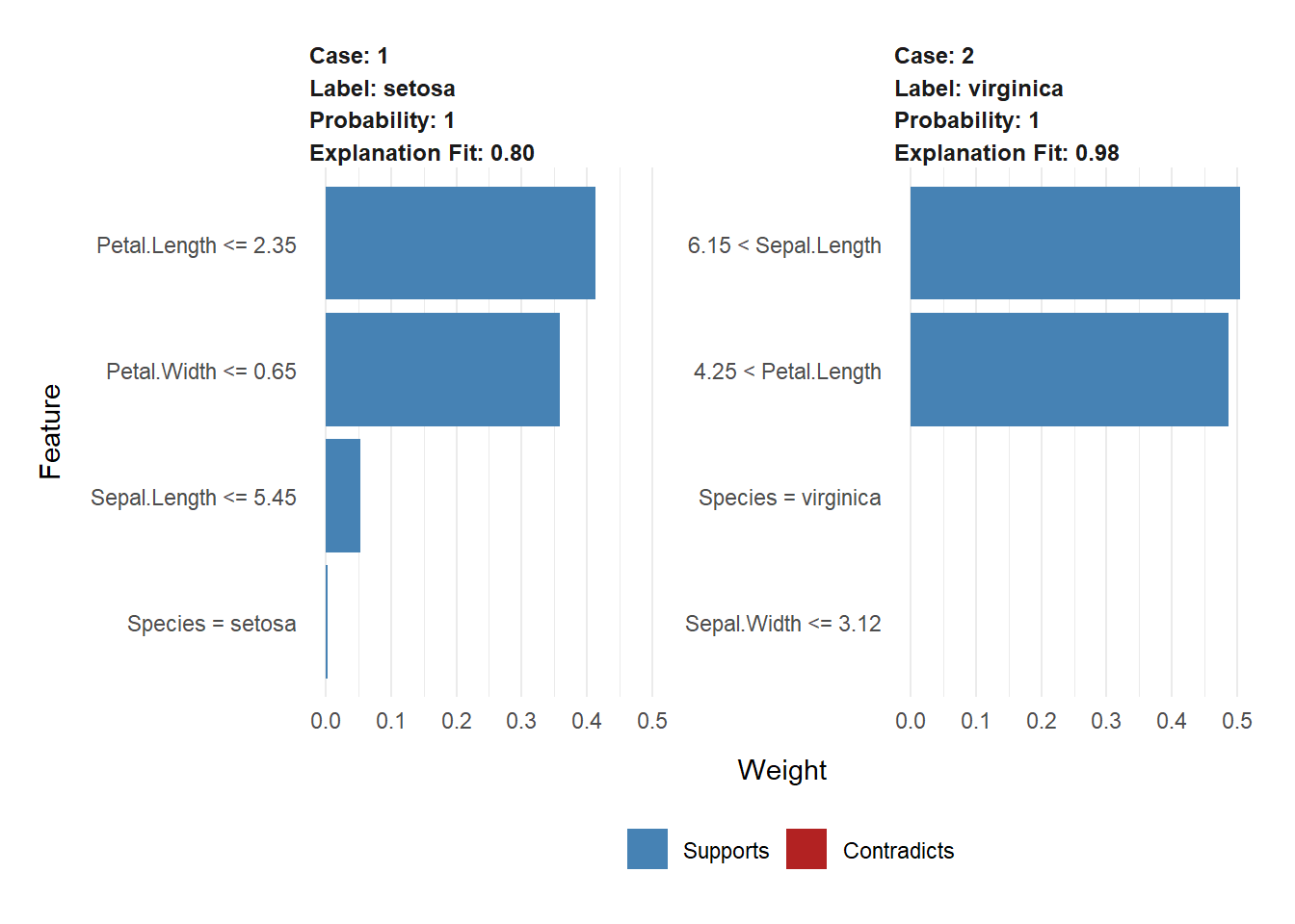
2          6.5         3.0          5.2         2.0 virginica

Explaining the prediction

Code

library(lime)
e <- lime(new_data, model, n_bins = 4)
explanation <- explain( x = new_data, 
                        explainer = e,n_labels = 1,
                        n_features = 4)
plot_features(explanation)