Support Vector Machines (SVM)

Introduction

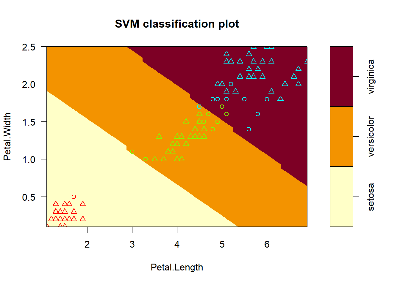
Support Vector Machines (SVM) are powerful supervised learning models used for classification and regression tasks. SVMs work by finding the hyperplane that best separates the classes in the feature space. R provides excellent packages like e1071 and caret to build and evaluate SVM models.

Key Steps in Building an SVM in R

Data Preparation: Cleaning and preparing data for analysis.

Model Training: Building the SVM model.

Model Evaluation: Assessing the model’s performance.

Prediction: Using the trained model to make predictions on new data.

Example: Predicting Species with SVM

Code

# install.packages("e1071")
# install.packages("caret")

library(e1071)
library(caret)
library(tidyverse)

Load and Prepare the Data

Code

# Load the data
data <- iris

# Split the data into training and testing sets
set.seed(123)
train_index <- createDataPartition(data$Species, p = 0.8, list = FALSE)
train_data <- data[train_index, ]
test_data <- data[-train_index, ]

Train the SVM Model

Code

# Train the model
model <- svm(Species ~ ., data = train_data, kernel = "linear")

# View the model summary
print(model)

Call:
svm(formula = Species ~ ., data = train_data, kernel = "linear")


Parameters:
   SVM-Type:  C-classification 
 SVM-Kernel:  linear 
       cost:  1 

Number of Support Vectors:  25

Ploting the Model

Code

plot(model, data = train_data,svSymbol = 1, dataSymbol = 2,Petal.Width ~ Petal.Length,
     slice = list(Sepal.Width = 3, Sepal.Length = 4),
     symbolPalette = rainbow(4))

Evaluate the Model

Assess the model’s performance on the testing set.

Code

# Make predictions on the testing set
predictions <- predict(model, newdata = test_data)

# Create a confusion matrix
conf_matrix <- confusionMatrix(predictions, test_data$Species)
print(conf_matrix)

Confusion Matrix and Statistics

            Reference
Prediction   setosa versicolor virginica
  setosa         10          0         0
  versicolor      0         10         1
  virginica       0          0         9

Overall Statistics
                                          
               Accuracy : 0.9667          
                 95% CI : (0.8278, 0.9992)
    No Information Rate : 0.3333          
    P-Value [Acc > NIR] : 2.963e-13       
                                          
                  Kappa : 0.95            
                                          
 Mcnemar's Test P-Value : NA              

Statistics by Class:

                     Class: setosa Class: versicolor Class: virginica
Sensitivity                 1.0000            1.0000           0.9000
Specificity                 1.0000            0.9500           1.0000
Pos Pred Value              1.0000            0.9091           1.0000
Neg Pred Value              1.0000            1.0000           0.9524
Prevalence                  0.3333            0.3333           0.3333
Detection Rate              0.3333            0.3333           0.3000
Detection Prevalence        0.3333            0.3667           0.3000
Balanced Accuracy           1.0000            0.9750           0.9500

Prediction on New Data

Use the tuned model to make predictions on new data.

Code

# New data for prediction
new_data <- data.frame(
  Sepal.Length = c(5.1, 6.5),
  Sepal.Width = c(3.5, 3.0),
  Petal.Length = c(1.4, 5.2),
  Petal.Width = c(0.2, 2.0)
)

# Predict species for new data
new_predictions <- predict(model, newdata = new_data)
new_predictions

        1         2 
   setosa virginica 
Levels: setosa versicolor virginica

SVM Regression

Code

library(mlbench)
# Boston Housing Data
data('BostonHousing')
mydata <- BostonHousing
head(mydata)

     crim zn indus chas   nox    rm  age    dis rad tax ptratio      b lstat
1 0.00632 18  2.31    0 0.538 6.575 65.2 4.0900   1 296    15.3 396.90  4.98
2 0.02731  0  7.07    0 0.469 6.421 78.9 4.9671   2 242    17.8 396.90  9.14
3 0.02729  0  7.07    0 0.469 7.185 61.1 4.9671   2 242    17.8 392.83  4.03
4 0.03237  0  2.18    0 0.458 6.998 45.8 6.0622   3 222    18.7 394.63  2.94
5 0.06905  0  2.18    0 0.458 7.147 54.2 6.0622   3 222    18.7 396.90  5.33
6 0.02985  0  2.18    0 0.458 6.430 58.7 6.0622   3 222    18.7 394.12  5.21
  medv
1 24.0
2 21.6
3 34.7
4 33.4
5 36.2
6 28.7

Splitting the data

Code

set.seed(123) 
ind <- sample(2, nrow(mydata), replace = T, prob = c(0.8, 0.2))
train <- mydata[ind == 1,]
test <- mydata[ind == 2,]

Fitting the model

Code

s <- svm(medv ~ ., data=train)
s

Call:
svm(formula = medv ~ ., data = train)


Parameters:
   SVM-Type:  eps-regression 
 SVM-Kernel:  radial 
       cost:  1 
      gamma:  0.07142857 
    epsilon:  0.1 


Number of Support Vectors:  274

Predictions

Code

b <- predict(s,  test)
test$predicted <- b
test %>% 
  select(medv,predicted) %>% head()

   medv predicted
4  33.4  29.80758
5  36.2  30.00990
8  27.1  18.34913
11 15.0  18.74011
16 19.9  19.50807
20 18.2  18.63947

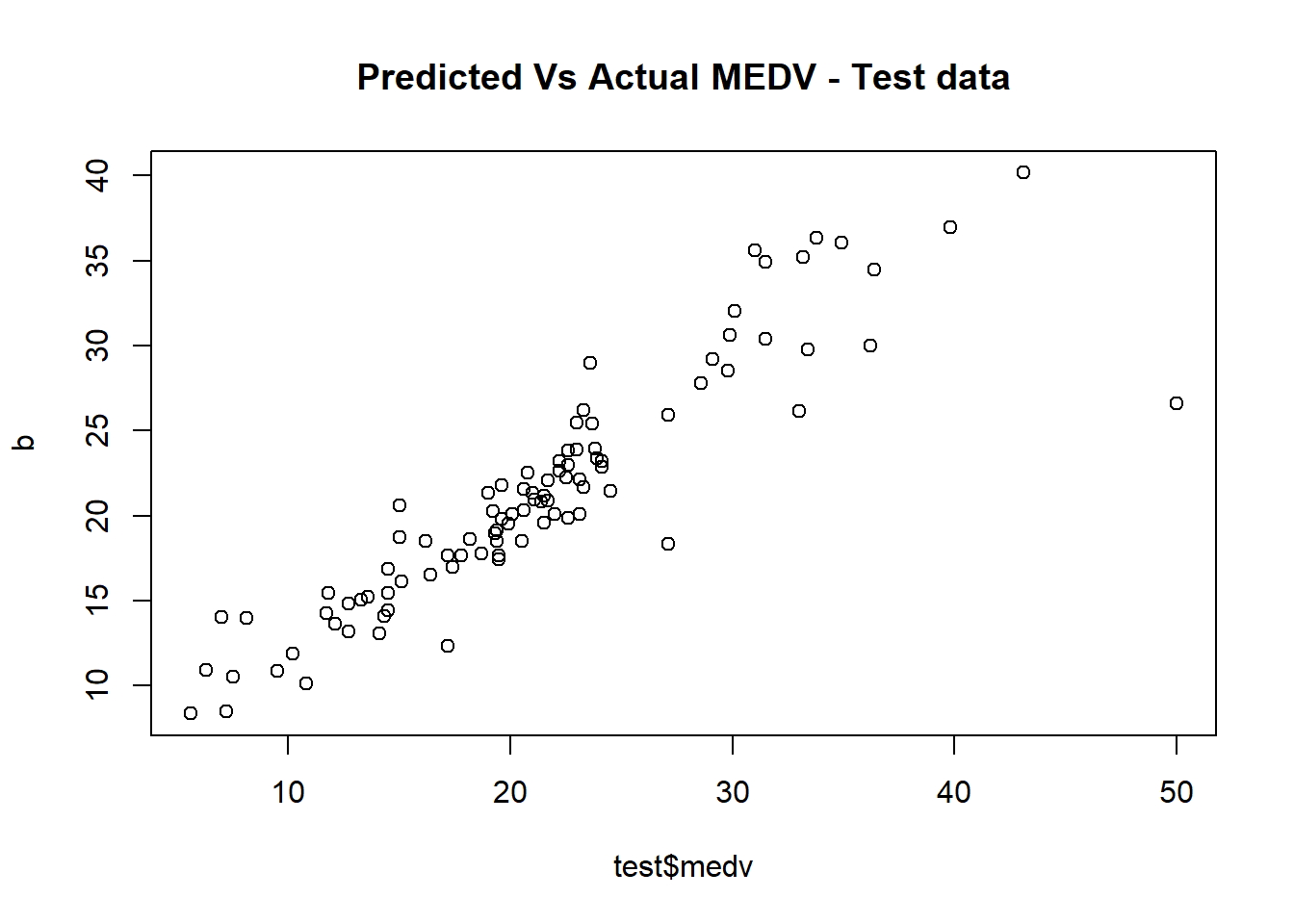
Scatter plot of Actual vs Predicted

Code

plot(b~ test$medv, main = 'Predicted Vs Actual MEDV - Test data')

RMSE & R Squared

Code

sqrt(mean((test$medv - b)^2))#RMSE

[1] 3.516934

Code

cor(test$medv, b) ^2# r squared

[1] 0.8204503