Introduction

Breast cancer remains a significant global health concern, affecting millions of individuals worldwide and posing formidable challenges to healthcare systems. Timely and accurate diagnosis is paramount in guiding treatment decisions and improving patient outcomes. This project delves into the realm of predictive modeling specifically focused on breast cancer diagnosis. By harnessing the power of machine learning and leveraging a rich dataset comprising clinical and diagnostic features, this endeavor aims to develop a robust predictive model capable of discerning between malignant and benign tumors with high accuracy.

Variables

Diagnosis: This categorical variable indicates the diagnosis outcome, with “M” representing malignant tumors and “B” representing benign tumors. It serves as the target variable for prediction.
Radius_mean, Texture_mean, Perimeter_mean: These variables represent the mean values of the radius, texture, and perimeter of the tumor cells, respectively, measured from diagnostic images.
Area_mean, Smoothness_mean, Compactness_mean, Concavity_mean, Concave_points_mean: These variables capture additional morphological characteristics of tumor cells, such as the area, smoothness, compactness, concavity, and number of concave points in the cell nuclei, averaged across the diagnostic images.
Symmetry_mean, Fractal_dimension_mean: These variables describe symmetry and fractal dimension features of tumor cells, providing insights into their structural complexity and irregularity.
Radius_se, Texture_se, Perimeter_se, Area_se, Smoothness_se, Compactness_se, Concavity_se, Concave_points_se, Symmetry_se, Fractal_dimension_se: These variables represent the standard error (SE) of the corresponding morphological features, providing information about the variability or uncertainty in their measurements.
Radius_worst, Texture_worst, Perimeter_worst, Area_worst, Smoothness_worst, Compactness_worst, Concavity_worst, Concave_points_worst, Symmetry_worst, Fractal_dimension_worst: These variables denote the “worst” or largest values of the respective morphological features observed in the tumor cells, providing insights into the most severe manifestations of tumor characteristics.

Required packages

Code

library(tidyverse)
library(randomForest)
library(janitor)
library(caret)
library(rsample)
library(DT)

Data Importation and Preprocessing

Code

cancer <- read_csv("breast-cancer.csv") %>% select(-id) %>% clean_names()
cancer$diagnosis <- factor(cancer$diagnosis)

Exploratory Data Analysis

Code

cancer %>% group_by(diagnosis) %>% 
  summarise(count = n()) %>% 
  ggplot(aes(diagnosis,count, label = count,fill = diagnosis))+geom_col()+geom_text(aes(label = count, vjust = 2))

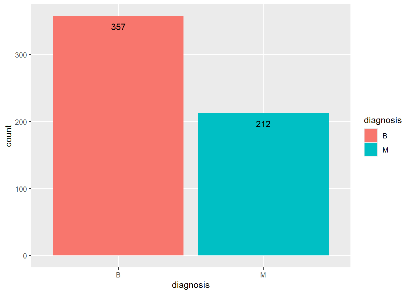
“B” indicates benign tumors. “M” indicates malignant tumors.

There are 357 instances of benign tumors (labelled as “B”). There are 212 instances of malignant tumors (labelled as “M”).

Checking for Dublicates

Code

cancer %>% duplicated() %>% unique()

[1] FALSE

There are no dublicates

Balancing the Data by Oversampling

Code

set.seed(123)

cancer <- upSample(cancer, cancer$diagnosis)
cancer <- cancer %>% select(-Class)
table(cancer$diagnosis)


  B   M 
357 357

The data is now balanced

Spliting the Data into Training and Testing

Code

set.seed(123)

split <- initial_split(cancer, prop = 0.8, strata = diagnosis)

train <- training(split)
test <- testing(split)
tabyl(cancer$diagnosis)

 cancer$diagnosis   n percent
                B 357     0.5
                M 357     0.5

Code

tabyl(train$diagnosis)

 train$diagnosis   n percent
               B 285     0.5
               M 285     0.5

Code

tabyl(test$diagnosis)

 test$diagnosis  n percent
              B 72     0.5
              M 72     0.5

Building a Randomforest Classification Model

Code

set.seed(123)
m1 <- caret::train(
  diagnosis~.,
  method = "rf", data = train,
  importance = T
)
m1

Random Forest 

570 samples
 30 predictor
  2 classes: 'B', 'M' 

No pre-processing
Resampling: Bootstrapped (25 reps) 
Summary of sample sizes: 570, 570, 570, 570, 570, 570, ... 
Resampling results across tuning parameters:

  mtry  Accuracy   Kappa    
   2    0.9654780  0.9308282
  16    0.9582624  0.9163916
  30    0.9527224  0.9052925

Accuracy was used to select the optimal model using the largest value.
The final value used for the model was mtry = 2.

Code

plot(m1)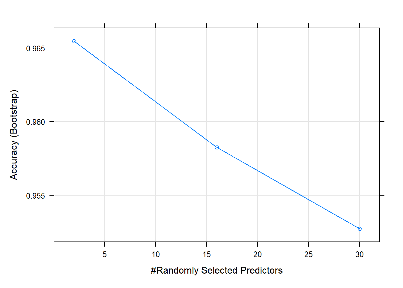

Variable Importance

Code

 v<- varImp(m1)
 v

rf variable importance

  only 20 most important variables shown (out of 30)

                        Importance
perimeter_worst             100.00
radius_worst                 96.34
concave_points_worst         91.77
texture_worst                88.20
area_worst                   85.11
concave_points_mean          80.29
concavity_worst              77.45
area_mean                    75.47
perimeter_mean               72.75
radius_mean                  69.84
area_se                      69.81
texture_mean                 68.16
concavity_mean               67.28
perimeter_se                 61.78
smoothness_worst             59.77
radius_se                    58.80
compactness_worst            51.80
symmetry_worst               50.13
fractal_dimension_worst      47.30
fractal_dimension_mean       43.47

Code

plot(v)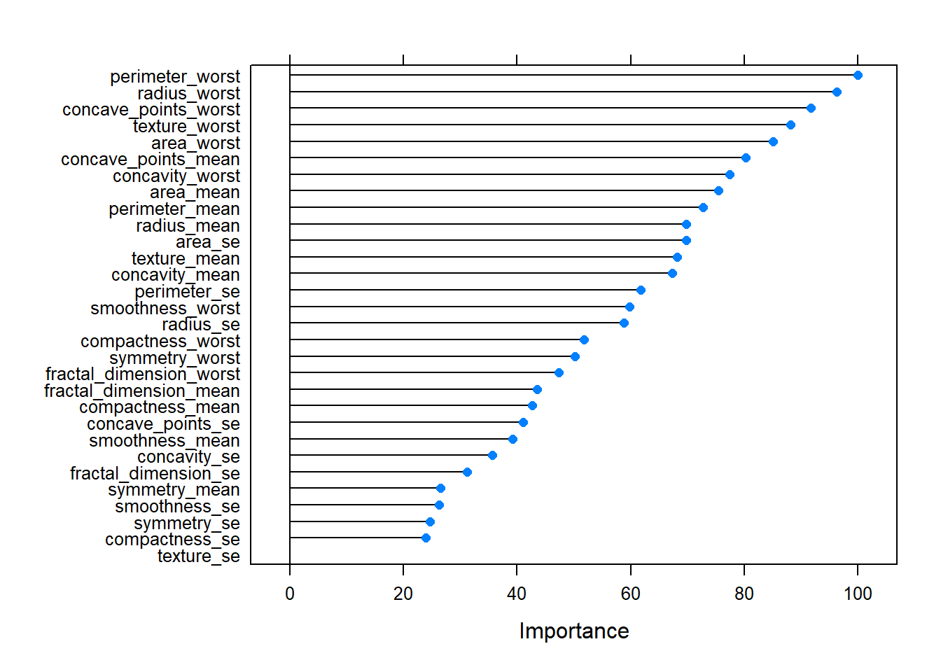

These values represent the importance of each predictor variable in contributing to the accuracy of the random forest model. Higher values suggest that the variable is more important in predicting the target variable (in this case, the diagnosis of breast cancer).

Predicting Using the Model

Code

p <- predict(m1 , newdata = test, type = "raw")
test$prediction <- p
head(p)

[1] B B B B B B
Levels: B M

The first five patients in the test data are predicted not to have cancer(Benign tumor)

Testing the Model Accuracy

Code

confusionMatrix(data = test$prediction, reference = test$diagnosis)

Confusion Matrix and Statistics

          Reference
Prediction  B  M
         B 70  0
         M  2 72
                                          
               Accuracy : 0.9861          
                 95% CI : (0.9507, 0.9983)
    No Information Rate : 0.5             
    P-Value [Acc > NIR] : <2e-16          
                                          
                  Kappa : 0.9722          
                                          
 Mcnemar's Test P-Value : 0.4795          
                                          
            Sensitivity : 0.9722          
            Specificity : 1.0000          
         Pos Pred Value : 1.0000          
         Neg Pred Value : 0.9730          
             Prevalence : 0.5000          
         Detection Rate : 0.4861          
   Detection Prevalence : 0.4861          
      Balanced Accuracy : 0.9861          
                                          
       'Positive' Class : B

Table of Predicted Against the Actual values

Code

test %>% select(diagnosis, prediction) %>% datatable()

Explaining the 1st 3 Prediction

Code

library(lime)
e <- lime(test[1:3,], m1, n_bins = 4)
explanation <- explain( x = test[1:3,], 
                        explainer = e,n_labels = 1,
                        n_features = 4)
b <- plot_features(explanation)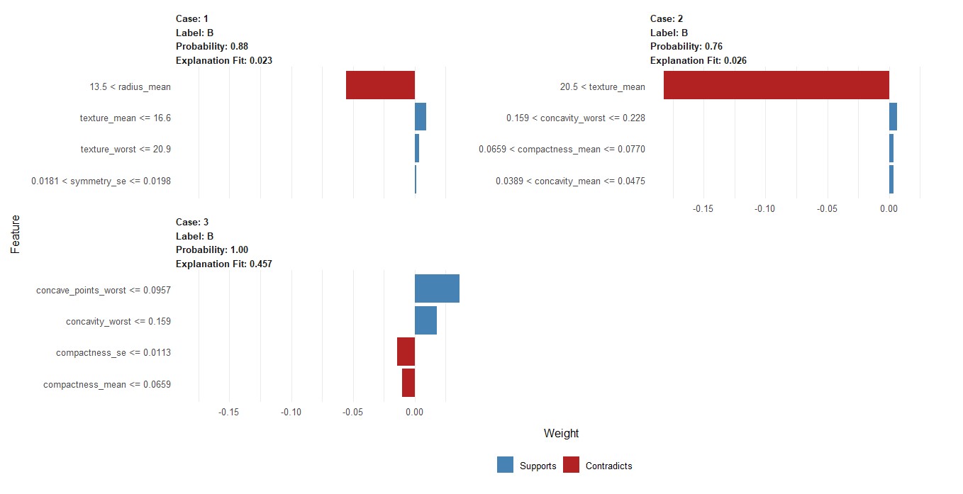

Limitation of the Model

Feature Selection: The predictive power of the model heavily relies on the choice of input features. While the current model considers various features such as radius, texture, perimeter, area, and others, there might be other relevant features not included in the analysis. Incorporating additional features or exploring feature engineering techniques could potentially enhance the model’s performance.

Model Interpretability: Random Forest models, like the one used here, are considered “black box” models, meaning they provide accurate predictions but offer limited interpretability. Understanding how individual features contribute to the model’s predictions can be challenging. Techniques such as feature importance analysis provide some insight but may not fully explain the underlying mechanisms driving the predictions.

External Factors: The model’s predictions may be influenced by factors not captured in the dataset, such as patient demographics, genetic factors, or environmental variables. Failing to account for these external factors could introduce bias or limit the model’s predictive accuracy in real-world applications.

Data source

Kaggle: link: https://www.kaggle.com/datasets/yasserh/breast-cancer-dataset