Introduction

In today’s dynamic real estate market, accurately predicting house prices is crucial for both buyers and sellers to make informed decisions. With the ever-changing landscape of property values influenced by various factors such as location, size, amenities, and market trends, leveraging data-driven insights becomes imperative.

This project aims to develop a predictive model for house prices utilizing machine learning techniques. By analyzing a comprehensive dataset encompassing key features like house area, number of bedrooms and bathrooms, amenities, and location attributes, the model seeks to forecast the selling price of residential properties.

The dataset comprises a diverse range of properties, each characterized by its unique set of features and corresponding market values. Leveraging advanced regression algorithms, I aim to uncover patterns and relationships within the data to accurately predict house prices.

Variables in the dataset

Price: This variable represents the selling price of a house in dollars. It is measured as an integer (e.g., 13300000, 12250000) and is the target variable in the predictive model, as we aim to predict house prices based on other features.
Area: This variable represents the area of the house in square feet. It is measured as an integer (e.g., 7420, 8960) and provides information about the size of the property.
Bedrooms: This variable represents the number of bedrooms in the house. It is measured as an integer (e.g., 4, 3) and provides information about the accommodation capacity of the property.
Bathrooms: This variable represents the number of bathrooms in the house. It is measured as an integer (e.g., 2, 4) and provides information about the sanitary facilities of the property.
Stories: This variable represents the number of stories or floors in the house. It is measured as an integer (e.g., 3, 4) and provides information about the vertical structure of the property.
Mainroad: This variable is categorical and indicates whether the house is located on a main road or not. It takes on binary values, such as “yes” or “no,” and provides information about the accessibility and potential traffic noise of the property.
Guestroom: This variable is categorical and indicates whether the house has a guestroom or not. It takes on binary values, such as “yes” or “no,” and provides information about additional accommodation features of the property.
Basement: This variable is categorical and indicates whether the house has a basement or not. It takes on binary values, such as “yes” or “no,” and provides information about additional storage or living space of the property.
Hotwaterheating: This variable is categorical and indicates whether the house has hot water heating or not. It takes on binary values, such as “yes” or “no,” and provides information about the heating system of the property.
Airconditioning: This variable is categorical and indicates whether the house has air conditioning or not. It takes on binary values, such as “yes” or “no,” and provides information about the cooling system of the property.
Parking: This variable represents the number of parking spaces available with the house. It is measured as an integer (e.g., 2, 3) and provides information about parking facilities for residents or visitors.
Prefarea: This variable is categorical and indicates whether the house is located in a preferred area or not. It takes on binary values, such as “yes” or “no,” and provides information about the desirability or popularity of the property’s location.
Furnishingstatus: This variable is categorical and indicates the furnishing status of the house. It can take on multiple values, such as “furnished,” “semi-furnished,” or “unfurnished,” and provides information about the interior condition and amenities of the property.

Required packages

Code

library(tidyverse)# for data manipulation
library(Boruta)# for feature selection
library(rsample)# for dividing my data into training and testing
library(performance)# evaluating the performance of the model
library(lava)
library(caret) #for data partitioning
library(DT)

Importing the dataset

Code

house <- read_csv("Housing.csv",col_names = T)

Data Pre-processing

Looking for dublicate

Code

house %>% duplicated() %>% unique()

[1] FALSE

There is no dublicate

Looking for incomplete cases

Code

house %>% filter(!complete.cases(.))

# A tibble: 0 × 13
# ℹ 13 variables: price <dbl>, area <dbl>, bedrooms <dbl>, bathrooms <dbl>,
#   stories <dbl>, mainroad <chr>, guestroom <chr>, basement <chr>,
#   hotwaterheating <chr>, airconditioning <chr>, parking <dbl>,
#   prefarea <chr>, furnishingstatus <chr>

Changing data types

Code

house$mainroad <- factor(house$mainroad)
house$guestroom <- factor(house$guestroom)
house$basement <- factor(house$basement)
house$hotwaterheating <- factor(house$hotwaterheating)
house$airconditioning <- factor(house$airconditioning)
house$prefarea <- factor(house$prefarea)
house$furnishingstatus <- factor(house$furnishingstatus)

Basic Exploratory Data Analysis

Code

house %>% summary()

     price               area          bedrooms       bathrooms    
 Min.   : 1750000   Min.   : 1650   Min.   :1.000   Min.   :1.000  
 1st Qu.: 3430000   1st Qu.: 3600   1st Qu.:2.000   1st Qu.:1.000  
 Median : 4340000   Median : 4600   Median :3.000   Median :1.000  
 Mean   : 4766729   Mean   : 5151   Mean   :2.965   Mean   :1.286  
 3rd Qu.: 5740000   3rd Qu.: 6360   3rd Qu.:3.000   3rd Qu.:2.000  
 Max.   :13300000   Max.   :16200   Max.   :6.000   Max.   :4.000  
    stories      mainroad  guestroom basement  hotwaterheating airconditioning
 Min.   :1.000   no : 77   no :448   no :354   no :520         no :373        
 1st Qu.:1.000   yes:468   yes: 97   yes:191   yes: 25         yes:172        
 Median :2.000                                                                
 Mean   :1.806                                                                
 3rd Qu.:2.000                                                                
 Max.   :4.000                                                                
    parking       prefarea        furnishingstatus
 Min.   :0.0000   no :417   furnished     :140    
 1st Qu.:0.0000   yes:128   semi-furnished:227    
 Median :0.0000             unfurnished   :178    
 Mean   :0.6936                                   
 3rd Qu.:1.0000                                   
 Max.   :3.0000

Explanation

Price:

Minimum: The lowest selling price of a house in the dataset is $1,750,000.

1st Quartile (Q1): 25% of the house prices are below $3,430,000.

Median: The median selling price (or the middle value) of houses in the dataset is $4,340,000.

Mean: The average selling price of houses in the dataset is approximately $4,766,729.

3rd Quartile (Q3): 75% of the house prices are below $5,740,000.

Maximum: The highest selling price of a house in the dataset is $13,300,000.

Area:

Minimum: The smallest house in the dataset has an area of 1,650 square feet.

1st Quartile (Q1): 25% of the houses have an area below 3,600 square feet.

Median: The median area of houses in the dataset is 4,600 square feet.

Mean: The average area of houses in the dataset is approximately 5,151 square feet.

3rd Quartile (Q3): 75% of the houses have an area below 6,360 square feet.

Maximum: The largest house in the dataset has an area of 16,200 square feet.

Bedrooms:

Minimum: The lowest number of bedroom in the dataset is 1.

1st Quartile (Q1): 25% of the houses have below 2 and below bedroom.

Median: The median number of bedrooms in the dataset is 3 bedroom.

3rd Quartile (Q3): 75% of the houses have 3 bedrooms and below.

Maximum: The largest number of bedroom in the dataset is 6.

Bathrooms

Minimum: The lowest number of bathrooms in the dataset is 1.

1st Quartile (Q1): 25% of the houses have 1 bathroom.

Median: The median number of bathrooms in the dataset is 1.

3rd Quartile (Q3): 75% of the houses have 2 and below bathrooms.

Maximum: The highest number of bathroom in the dataset is 4.

Stories:

Minimum: The lowest number of stories in the dataset is 1.

1st Quartile (Q1): 25% of the houses have 1 story.

Median: The median number of stories in the dataset is 2.

3rd Quartile (Q3): 75% of the houses have 2 and below storiess.

Maximum: The highest number of stories in the dataset is 4.

Mainroad:

77 houses are not located near a mainroad

468 houses are located near a mainroad

Guestroom

354 houses do nt have a guestroom

97 houses have guestroom

Basement

354 houses do not have a basement

191 houses has a basement

Hotwaterheating

520 houses do not have hot water heating

25 houses have water heating

Air conditioning

373 houses do not have air conditioning

172 houses have air conditioning

Preferred area

417 houses are not in a preferred area

128 houses are in a preferred area

Furnishing status:

140 houses in the dataset are furnished

227 houses are semi-furnished

178 houses are unfurnished

Histogram of price

Code

house %>% ggplot(aes(price, fill = "red"))+geom_histogram(color = "blue")+theme(
  legend.position = "none"
)

`stat_bin()` using `bins = 30`. Pick better value with `binwidth`.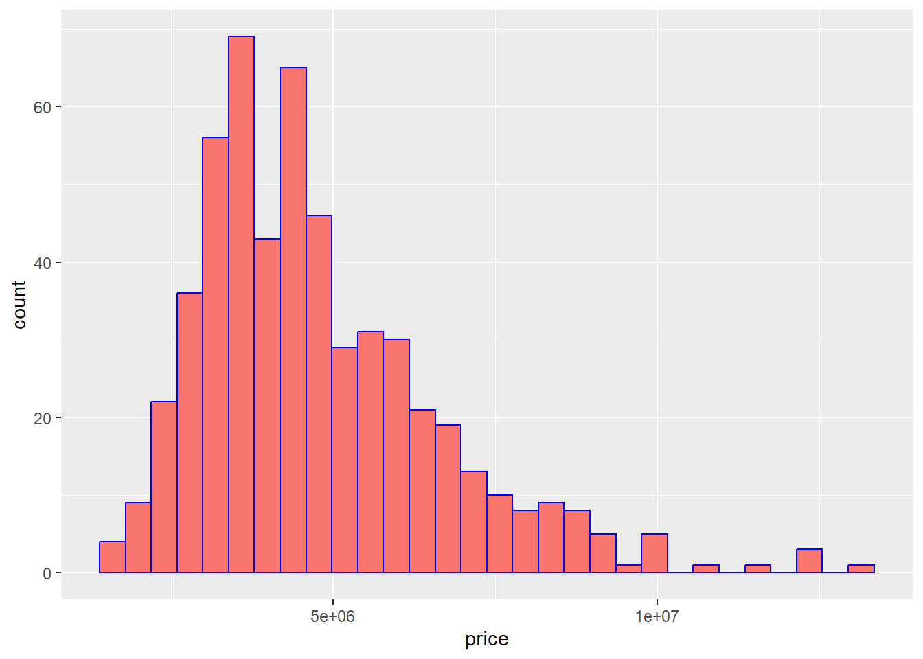

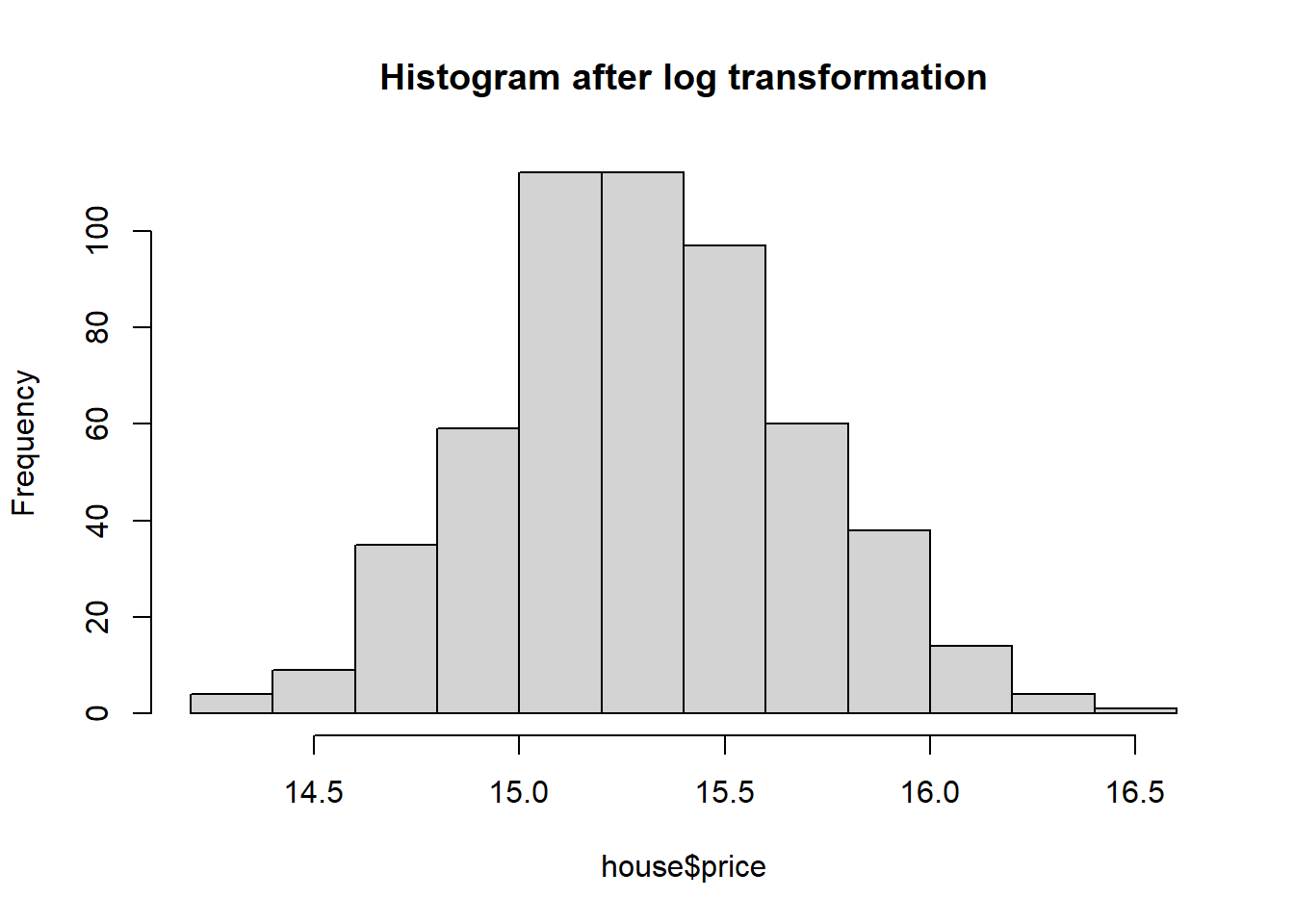
The dependent variable(Price) is not normally distributed

Transformation of our dependent variable

Code

house$price <- log(house$price)
house$area<- log(house$area)
hist(house$price,main = "Histogram after log transformation")

Splitting the Data

Code

set.seed(1)
s <- initial_split(house, prop = 0.90)
train <- training(s)
test <- testing(s)

Multiple linear Regression

Code

library(robustbase)
m <- lmrob(price ~ .,data = train)
sjPlot::tab_model(m, digits = 3, show.intercept = FALSE)

	price
Predictors	Estimates	CI	p
area	0.294	0.240 – 0.349	<0.001
bedrooms	0.022	-0.007 – 0.052	0.137
bathrooms	0.170	0.125 – 0.215	<0.001
stories	0.086	0.062 – 0.110	<0.001
mainroad [yes]	0.090	0.036 – 0.143	0.001
guestroom [yes]	0.061	0.007 – 0.116	0.027
basement [yes]	0.093	0.045 – 0.142	<0.001
hotwaterheating [yes]	0.141	0.018 – 0.265	0.025
airconditioning [yes]	0.155	0.112 – 0.197	<0.001
parking	0.033	0.010 – 0.057	0.005
prefarea [yes]	0.138	0.096 – 0.180	<0.001
furnishingstatus [semi-furnished]	-0.009	-0.051 – 0.033	0.675
furnishingstatus [unfurnished]	-0.114	-0.165 – -0.063	<0.001
Observations	490
R² / R² adjusted	0.728 / 0.720

Interpretation of Significant variables

Area: A 1% increase in the area of the house corresponds to a 29.4% increase in the price of the house.
Bathrooms: Each additional bathroom is associated with an approximate 17% increase in the house price.
Stories: Each additional story in the house corresponds to an approximate 8.6% increase in the house price.
Mainroad (Yes): Houses located on the main road tend to have prices higher by approximately 9% compared to those not on the main road.
Guestroom (Yes): Houses with a guestroom have prices higher by approximately 6% compared to those without a guestroom.
Basement (Yes): Similarly, houses with a basement tend to have prices higher by approximately 9.3% compared to those without.
Hotwaterheating (Yes): Houses with hot water heating have prices higher by approximately 14.1% compared to those without.
Airconditioning (Yes): Similarly, houses with air conditioning tend to have prices higher by approximately 15.5% compared to those without.
Parking: Each additional parking space is associated with an approximate 3.3% increase in the house price.
Prefarea (Yes): Houses in preferred areas have prices higher by approximately 13.8% compared to those not in preferred areas.
Furnishing Status (Unfurnished): Unfurnished houses tend to have prices lower by approximately 11.4% compared to furnished ones.
Adjusted R squared in my model is 72 percent meaning that my model explain 72 percent of variation in house prices. 28 percent is explained by other factors that are not in the model.

Diagnostic Tests

1)Auto correlation

Code

a <- check_autocorrelation(m)
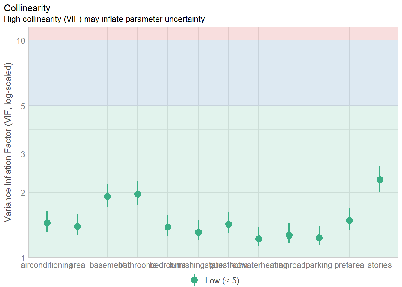
a

OK: Residuals appear to be independent and not autocorrelated (p = 0.162).

2) Multcolinearity

Code

mc <- check_collinearity(m)
plot(mc)

Variable `Component` is not in your data frame :/

3) Homoscedasticity

Code

h <- check_heteroscedasticity(m)
plot(h)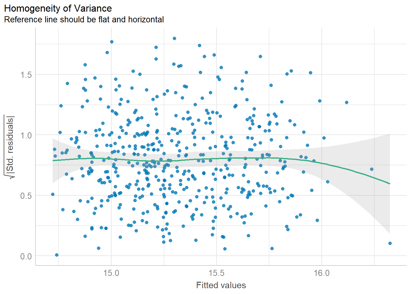

4) Normality test

Code

n <- data.frame(res = m$residuals)
hist(n$res, col = "red", main = "Histogram of regression residuals")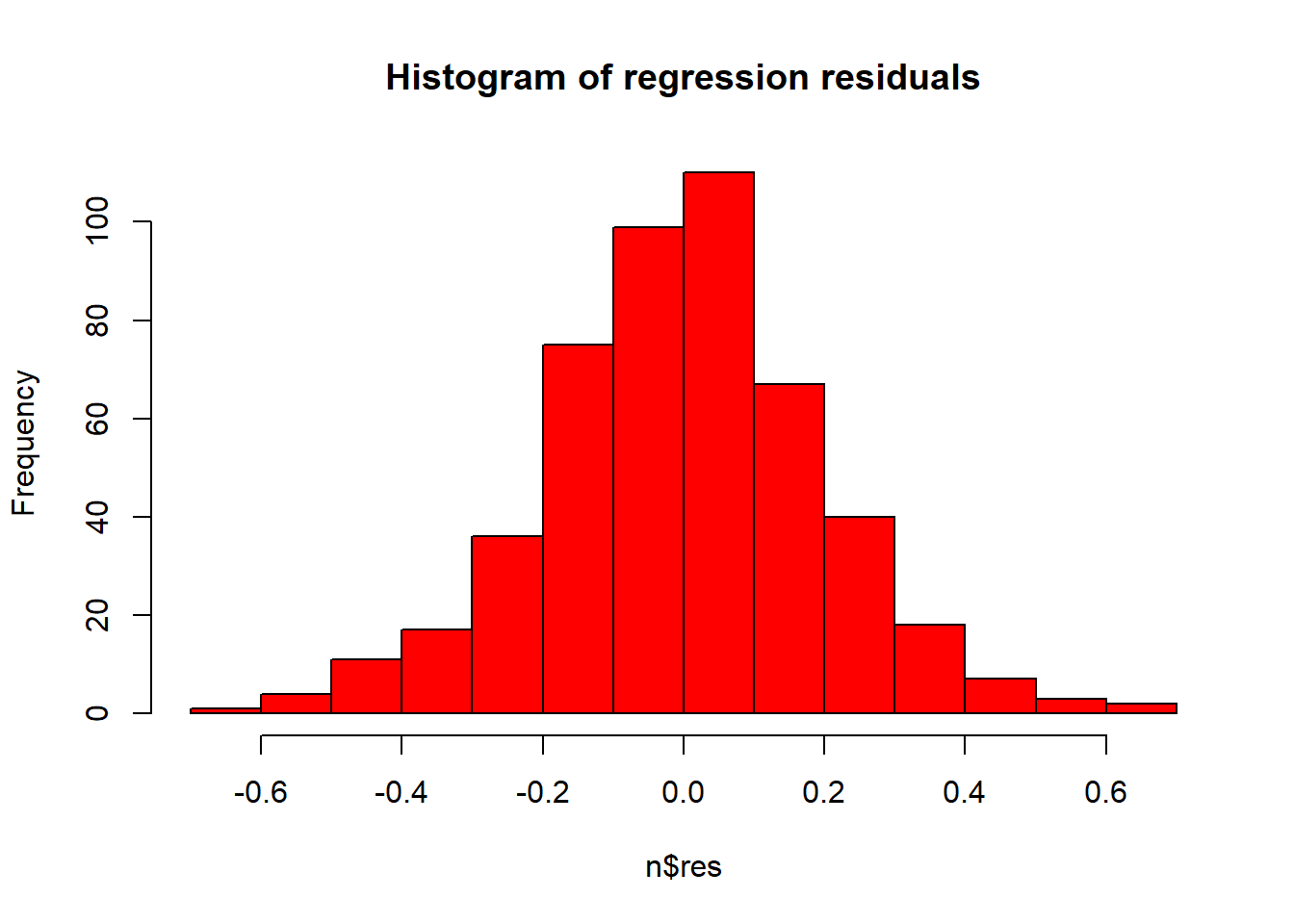

Predicting Using The Model

Code

pred <- predict(m,newdata = test,type = "response")
prediction <- exp(pred)

Code

test$prediction <- prediction
test %>% mutate(Actual_price = round(exp(price)),0) %>% select(-1,predicted_price=prediction,Actual_price,everything()) %>% 
  select(Actual_price,predicted_price) %>% 
  mutate(predicted_price = round(predicted_price,0)) %>% 
  datatable()

Limitation of my model

Limited Features:Even though there are no missing values, the dataset may still lack some important features that could affect house prices. Features like neighborhood amenities, crime rates, or access to public transportation could significantly impact house prices but are not be included in the dataset.
Data Bias:The dataset may be biased towards certain types of houses or neighborhoods, which could affect the model’s ability to generalize to other areas or housing markets. For example, if the dataset predominantly includes houses from affluent neighborhoods, the model’s predictions may not be accurate for houses in lower-income areas.
The dataset may not reflect current market conditions or trends. Changes in the housing market over time, such as shifts in demand, economic conditions, or regulatory changes, may not be captured in the dataset, potentially affecting the model’s predictive performance. Geographic Specificity:
The dataset may represent a specific geographic region or market, limiting the model’s generalizability to houses in other regions with different market dynamics and socioeconomic factors. External Factors:
External factors like economic conditions, government policies, or natural disasters may influence house prices but may not be accounted for in the dataset. Ignoring these external factors could limit the accuracy and reliability of the model predictions. Evaluation Metrics:

Datasource:

Kaggle

link : https://www.kaggle.com/datasets/yasserh/housing-prices-dataset