Loan Approval Prediction

Introduction

Dream Housing Finance company deals in all kinds of home loans. They have presence across all urban, semi urban and rural areas. Customer first applies for home loan and after that company validates the customer eligibility for loan. Company wants to automate the loan eligibility process (real time) based on customer detail provided while filling online application form. These details are Gender, Marital Status, Education, Number of Dependents, Income, Loan Amount, Credit History and others. To automate this process, they have provided a dataset to identify the customers segments that are eligible for loan amount so that they can specifically target these customers.

Overview of the Project

The primary objective of this project is to develop a robust loan eligibility prediction system utilizing machine learning techniques. By leveraging historical data on loan applications and their outcomes, I aim to construct models capable of classifying whether a loan application should be accepted or rejected.

Objective of the Project

The overarching goal of this project is twofold:

• To facilitate more informed decision-making for financial institutions by providing them with a reliable tool for assessing loan eligibility.

• To enhance the borrowing experience for clients by ensuring fair and transparent evaluation of loan applications, thereby fostering trust and satisfaction.

Importance of Loan Eligibility Prediction

• Risk Management: By accurately assessing the creditworthiness of applicants, financial institutions can mitigate the risk of default and minimize potential financial losses.

• Efficiency Enhancement: Automated loan eligibility prediction systems streamline the application review process, reducing manual labor and operational costs while improving efficiency.

• Customer Satisfaction: Transparent and equitable evaluation of loan applications enhances customer satisfaction, fostering long-term relationships and loyalty.

• Compliance Requirements: Adherence to regulatory guidelines and compliance standards necessitates thorough assessment of loan applicants to ensure fair lending practices.

Variables in the Dataset

Description of the Data

Variable	Description
Loan_ID	Unique Loan ID
Gender	Male/ Female
Married	Applicant married (Y/N)
Dependents	Number of dependents
Education	Applicant Education (Graduate/ Under Graduate)
Self_Employed	Self employed (Y/N)
ApplicantIncome	Applicant income
CoapplicantIncome	Coapplicant income
LoanAmount	Loan amount in thousands
Loan_Amount_Term	Term of loan in months
Credit_History	credit history meets guidelines
Property_Area	Urban/ Semi Urban/ Rural
Loan_Status	(Target) Loan approved (Y/N)

Packages Used

Code

library(tidyverse)
library(caret)
library(rsample)
library(randomForest)
library(janitor)
library(rpart)
library(lime)
library(DT)

Data Importation

Code

loan <- read.csv("Loan_Data.csv")%>% tibble()

Data Preprocessing

Code

# Replace empty strings with NA in specific columns
loan <- loan %>%
  mutate(Gender = na_if(Gender, ""),
    Married = na_if(Married, ""),
    Dependents = na_if(Dependents, ""),
    Education = na_if(Education, ""),
    Self_Employed = na_if(Self_Employed, ""),
    Loan_ID = na_if(Loan_ID, ""),
    Property_Area = na_if(Property_Area, ""),
    Loan_Status = na_if(Loan_Status, "")
  )
loan <- loan %>% filter(complete.cases(.))
library(dplyr)

# Convert specified columns to factors
loan$Gender <- factor(loan$Gender)
loan$Married <- factor(loan$Married)
loan$Dependents <- factor(loan$Dependents)
loan$Education <- factor(loan$Education)
loan$Self_Employed <- factor(loan$Self_Employed)
loan$Loan_Amount_Term <- factor(loan$Loan_Amount_Term)
loan$Credit_History <- factor(loan$Credit_History)
loan$Property_Area <- factor(loan$Property_Area)
loan$Loan_Status <- factor(loan$Loan_Status)


loan <- loan %>% select(-1)

Explroratory Data Analysis

Gender Distribution in Loan Applications

Code

#EDA
theme_set(theme_classic())
loan %>% group_by(Gender) %>% 
  summarise(count = n()) %>% 
  ggplot(aes(Gender,count, fill = Gender))+geom_col()+theme(
    legend.position = "none"
  )+labs(
    y = "Count"
  )+geom_label(aes(label = count))

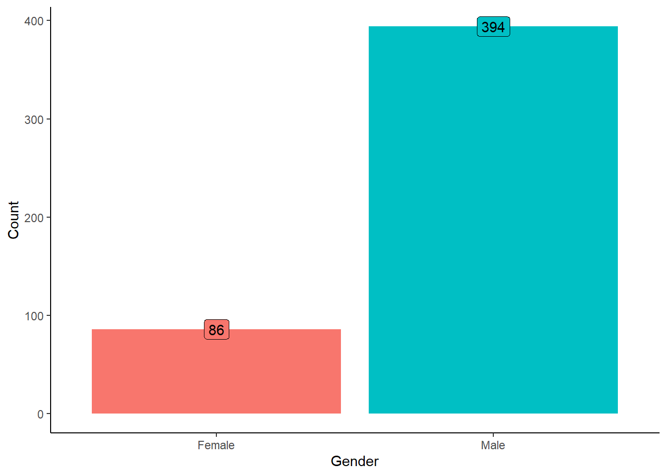
Out of the total applications analyzed, 86 were from Females, while over 394 were from males. This gender distribution underscores the importance of further investigating potential factors influencing borrowing behavior among different demographic groups.

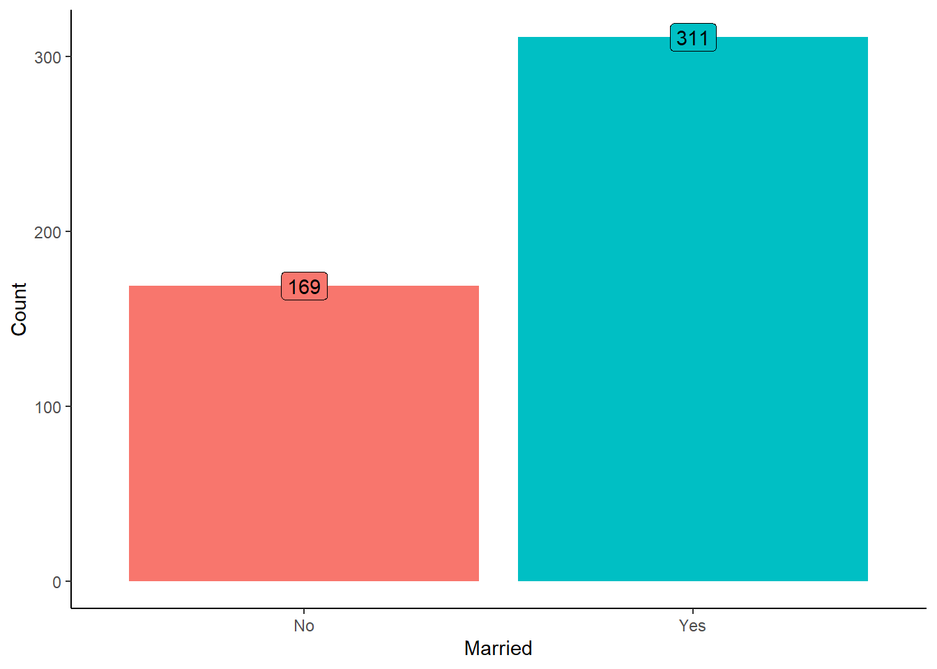
Marital Status Distribution in Loan Applications

Code

loan %>% group_by(Married) %>% 
  summarise(count = n()) %>% 
  ggplot(aes(Married,count, fill = Married))+geom_col()+theme(
    legend.position = "none"
  )+labs(
    y = "Count"
  )+geom_label(aes(label = count))

Distribution of Number of Dependents in Loan Applications

Code

loan %>% group_by(Dependents) %>% 
  summarise(count = n()) %>% 
  ggplot(aes(Dependents,count, fill = Dependents))+geom_col()+theme(
    legend.position = "none"
  )+labs(
    y = "Count")+geom_label(aes(label = count))

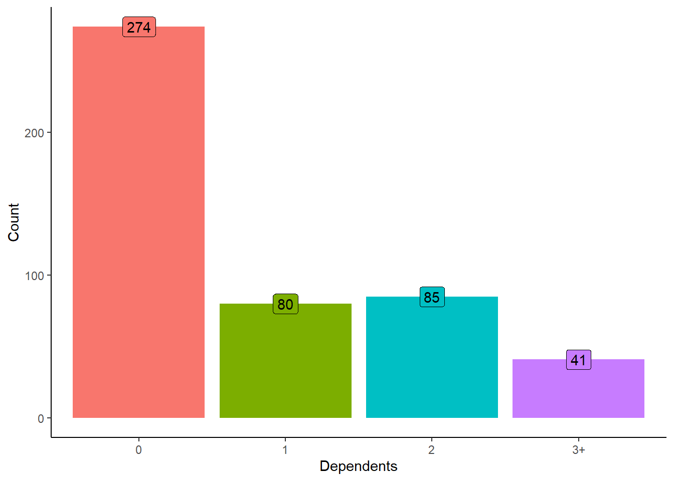
Understanding the distribution of dependents among applicants is essential for assessing their financial responsibilities and potential impact on loan repayment capabilities.

Educational Background Distribution in Loan Applications

Code

loan %>% group_by(Education) %>% 
  summarise(count = n()) %>% 
  ggplot(aes(Education,count, fill = Education))+geom_col()+theme(
    legend.position = "none"
  )+labs(
    y = "Count")+geom_label(aes(label = count))

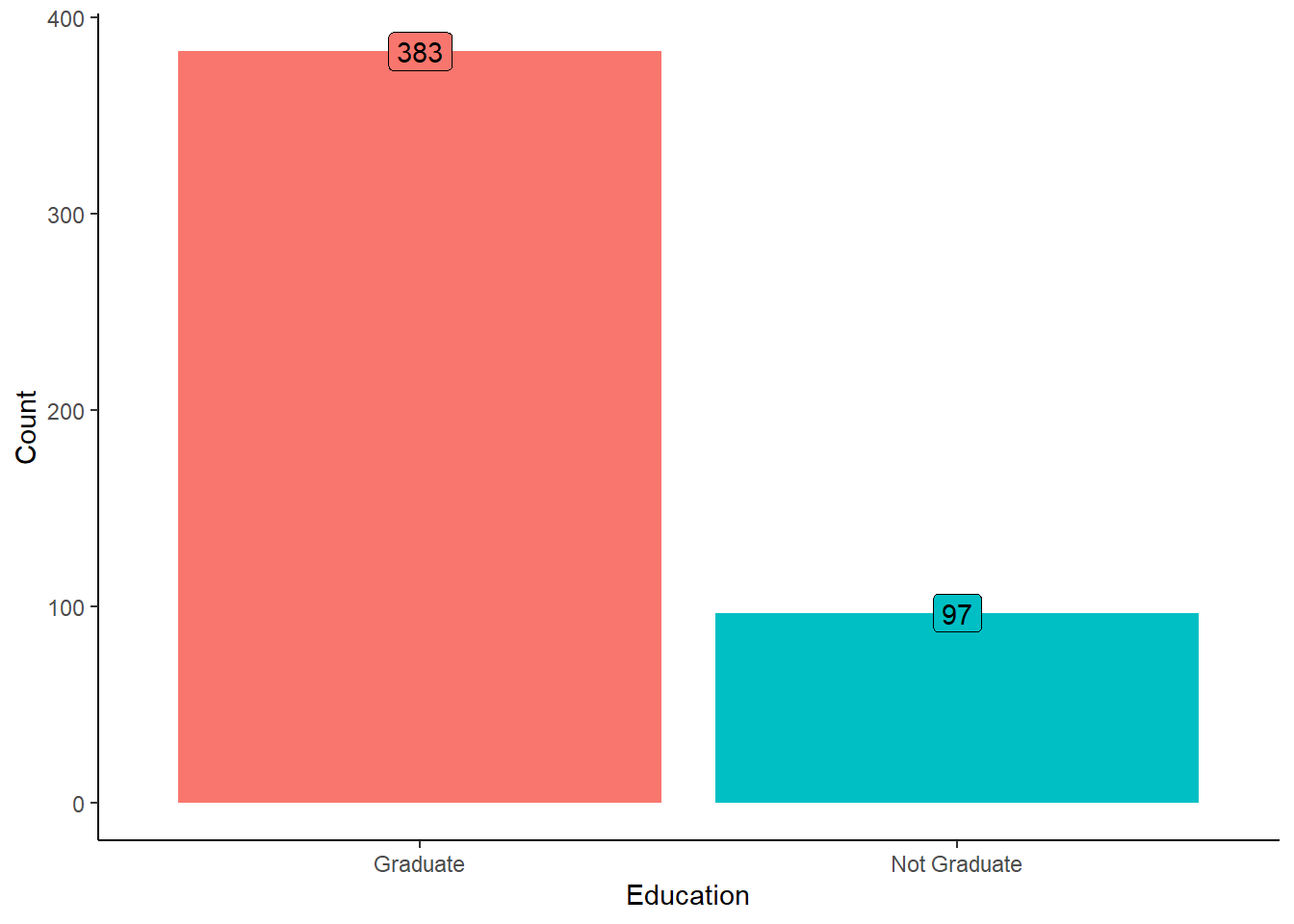
Understanding the educational background of applicants is crucial as it may correlate with factors such as income level, employment opportunities, and financial literacy, all of which influence loan eligibility and repayment capabilities.

Self-Employment Status Distribution in Loan Applications

Code

loan %>% group_by(Self_Employed) %>% 
  summarise(count = n()) %>% 
  ggplot(aes(Self_Employed,count, fill = Self_Employed))+geom_col()+theme(
    legend.position = "none"
  )+labs(
    y = "Count")+geom_label(aes(label = count))

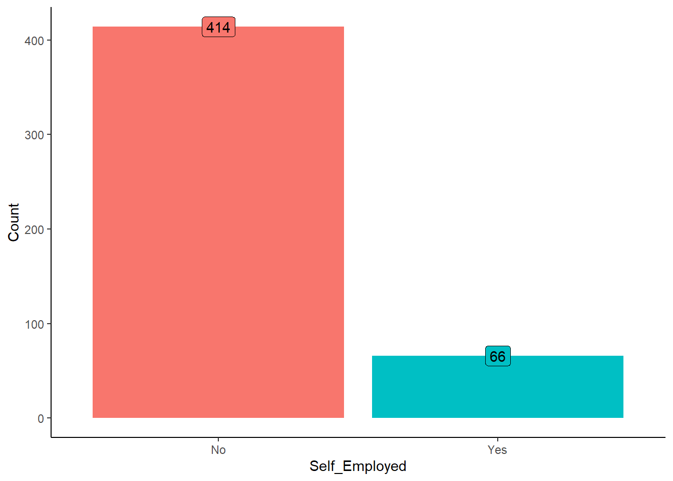
The proportion of self-employed applicants provides insights into the diversity of employment types within the applicant pool and may influence risk assessment and loan approval decisions.

Distribution of Loan Amount Terms in Loan Applications

Code

loan %>% group_by(Loan_Amount_Term) %>% 
  summarise(count = n()) %>% 
  ggplot(aes(Loan_Amount_Term,count, fill = Loan_Amount_Term))+geom_col()+theme(
    legend.position = "none"
  )+labs(
    y = "Count", x = "Duration of Payment")+geom_label(aes(label = count))

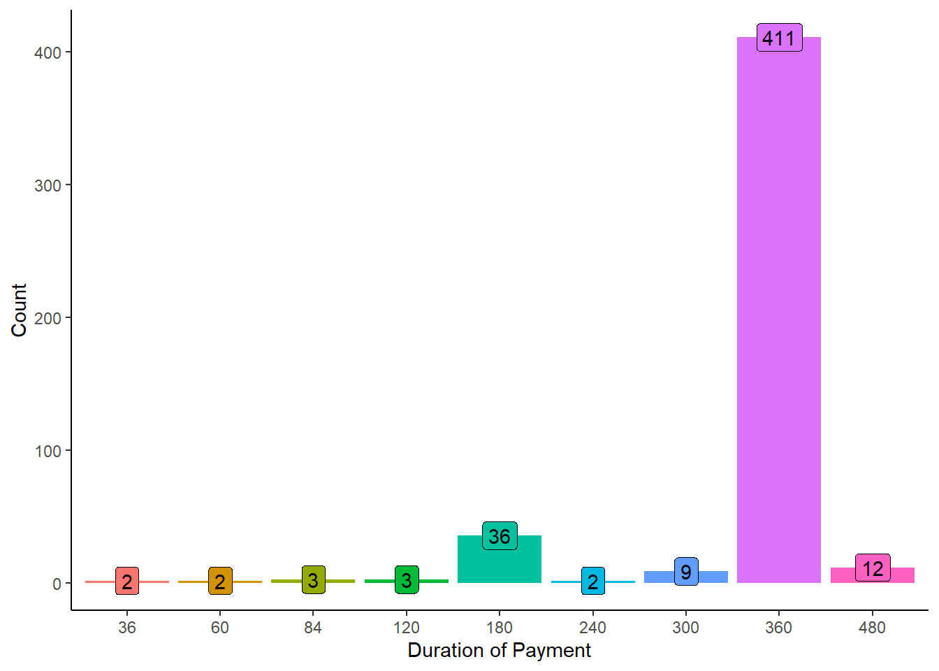
The analysis reveals that the majority of loan applications, the highest number, were for a loan term of 360 months (30 years). As the loan term decreases, the number of applications decreases accordingly. This distribution indicates a preference among applicants for longer loan terms, potentially reflecting their financial planning and repayment capabilities.

Distribution of Credit History in Loan Applications

Code

c <- loan %>% select(Credit_History) 
c$Credit_History <- factor(c$Credit_History, levels =c(0,1), labels = c("No","Yes"))
  
c %>% group_by(Credit_History) %>% 
  summarise(count = n()) %>% 
  ggplot(aes(Credit_History,count, fill = Credit_History))+geom_col()+theme(
    legend.position = "none"
  )+labs(y = "Count", x = "Credit History")+geom_label(aes(label = count))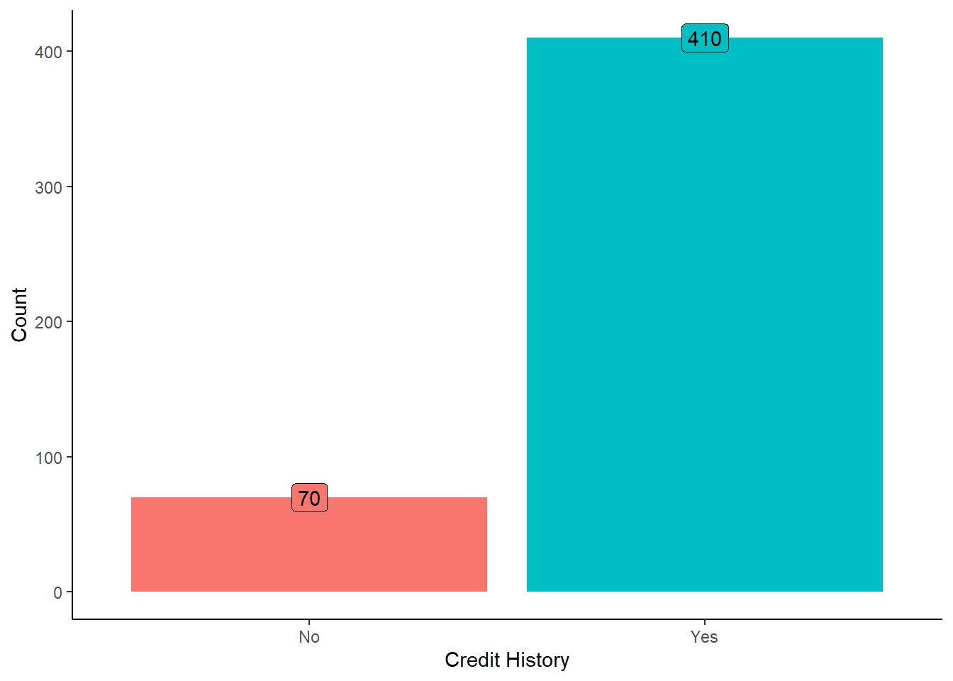

Understanding the distribution of credit history among applicants is crucial as it serves as a key factor in assessing their creditworthiness and likelihood of loan repayment.

Distribution of Property Area in Loan Applications

Code

loan %>% group_by(Property_Area) %>% 
  summarise(count = n()) %>% 
  ggplot(aes(Property_Area,count, fill = Property_Area))+geom_col()+theme(
    legend.position = "none"
  )+labs(
    y = "Count", x = "Property Area")+geom_label(aes(label = count))

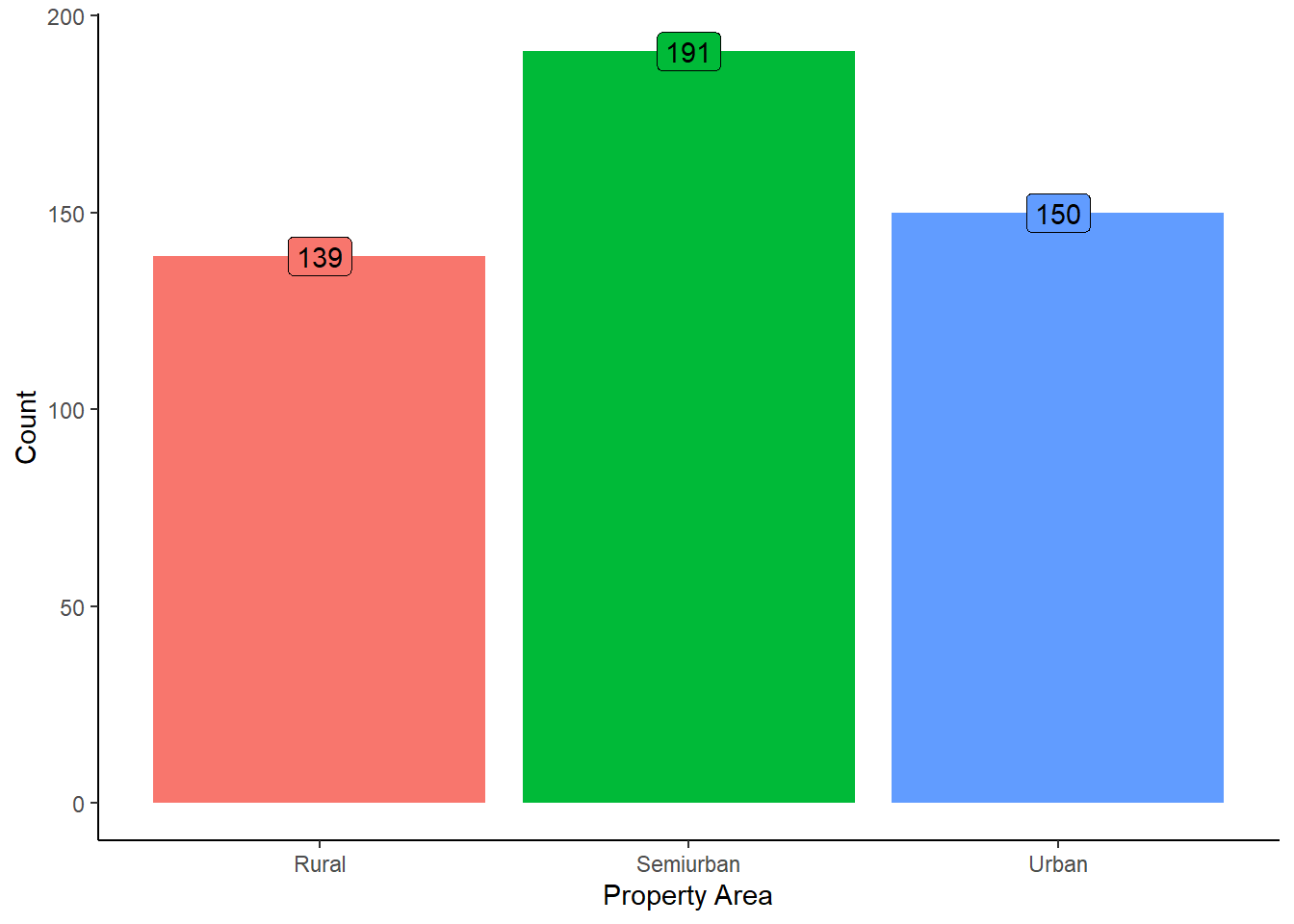
Understanding the distribution of property areas provides insights into the geographic preferences of loan applicants and may correlate with factors such as lifestyle, employment opportunities, and property values.

Loan Status Distribution in Loan Applications

Code

loan %>% group_by(Loan_Status) %>% 
  summarise(count = n()) %>% 
  ggplot(aes(Loan_Status,count, fill = Loan_Status))+geom_col()+theme(
    legend.position = "none"
  )+labs(
    y = "Count")+geom_label(aes(label = count))

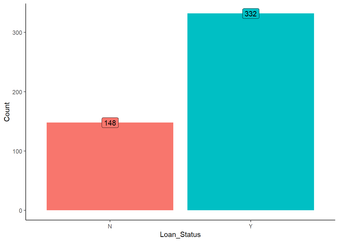
Among the analyzed loan applications, 332 were approved (labeled as “Y”), while 148 were rejected (labeled as “N”).

Data Partitioning: Splitting the Dataset for Training and Testing

• Training Data

The training set comprises a portion of the original dataset, typically the majority, and is used to train the machine learning model.This subset contains labeled examples, where both the input features and the corresponding target variable (in this case, loan status) are provided.During the training phase, the model learns patterns and relationships within the data, adjusting its parameters to minimize the prediction error.The model is exposed to the training data multiple times through iterations or epochs, optimizing its performance on the task at hand.

• Testing Data

The testing set is a separate portion of the dataset reserved exclusively for evaluating the trained model’s performance. This subset also contains labeled examples, but the model has not seen these examples during the training phase. Once the model has been trained on the training data, it is evaluated on the testing data to assess its generalization capability, i.e., how well it performs on unseen data. The testing set provides an unbiased estimate of the model’s performance and helps identify potential issues such as overfitting (when the model learns to memorize the training data rather than generalize from it).

Code

set.seed(1)
loan <- upSample(loan, loan$Loan_Status)
loan <- loan %>% select(-Class)
split_loan <- initial_split(loan, prop = 0.8, strata = Loan_Status)
loan_train <- training(split_loan)
loan_test <- testing(split_loan)

Code

tabyl(loan_test$Loan_Status)

 loan_test$Loan_Status  n percent
                     N 67     0.5
                     Y 67     0.5

Code

tabyl(loan_train$Loan_Status)

 loan_train$Loan_Status   n percent
                      N 265     0.5
                      Y 265     0.5

Model Selection: Choosing the Best Algorithm for Loan Eligibility Prediction

Random Forest Model

Code

cvcontrol <- trainControl(method="repeatedcv", 
                          number = 5,
                          repeats = 2,
                          allowParallel=TRUE)
set.seed(1) 

forest <- train(Loan_Status ~., data = loan_train,
                method="rf",
                trControl=cvcontrol,
                importance=TRUE)

Model accuracy

Code

#prediction
p1  <- predict(forest, newdata = loan_test)
confusionMatrix(p1, reference = loan_test$Loan_Status, positive = "Y")

Confusion Matrix and Statistics

          Reference
Prediction  N  Y
         N 60  7
         Y  7 60
                                          
               Accuracy : 0.8955          
                 95% CI : (0.8309, 0.9417)
    No Information Rate : 0.5             
    P-Value [Acc > NIR] : <2e-16          
                                          
                  Kappa : 0.791           
                                          
 Mcnemar's Test P-Value : 1               
                                          
            Sensitivity : 0.8955          
            Specificity : 0.8955          
         Pos Pred Value : 0.8955          
         Neg Pred Value : 0.8955          
             Prevalence : 0.5000          
         Detection Rate : 0.4478          
   Detection Prevalence : 0.5000          
      Balanced Accuracy : 0.8955          
                                          
       'Positive' Class : Y               
                                          

Decision Tree Model

Code

library(party)
set.seed(1)
tree_model <- train(Loan_Status ~ ., 
            data = loan_train,
            method = "ctree", 
            trControl = cvcontrol)
trP2 <- predict(tree_model,newdata = loan_test,type = "raw")
confusionMatrix(trP2, reference = loan_test$Loan_Status, positive = "Y")

Confusion Matrix and Statistics

          Reference
Prediction  N  Y
         N 42 11
         Y 25 56
                                         
               Accuracy : 0.7313         
                 95% CI : (0.648, 0.8042)
    No Information Rate : 0.5            
    P-Value [Acc > NIR] : 4.055e-08      
                                         
                  Kappa : 0.4627         
                                         
 Mcnemar's Test P-Value : 0.03026        
                                         
            Sensitivity : 0.8358         
            Specificity : 0.6269         
         Pos Pred Value : 0.6914         
         Neg Pred Value : 0.7925         
             Prevalence : 0.5000         
         Detection Rate : 0.4179         
   Detection Prevalence : 0.6045         
      Balanced Accuracy : 0.7313         
                                         
       'Positive' Class : Y              
                                         

Logistic regression

Code

logit <- glm(Loan_Status ~., data = loan_train, family = "binomial")
l_p <- predict(logit, newdata = loan_test, type = "response")
l_p<- ifelse(l_p > 0.5, "Y","N")
l_p <- factor(l_p)
confusionMatrix(l_p, reference = loan_test$Loan_Status, positive = "Y")

Confusion Matrix and Statistics

          Reference
Prediction  N  Y
         N 42 18
         Y 25 49
                                         
               Accuracy : 0.6791         
                 95% CI : (0.593, 0.7571)
    No Information Rate : 0.5            
    P-Value [Acc > NIR] : 2.056e-05      
                                         
                  Kappa : 0.3582         
                                         
 Mcnemar's Test P-Value : 0.3602         
                                         
            Sensitivity : 0.7313         
            Specificity : 0.6269         
         Pos Pred Value : 0.6622         
         Neg Pred Value : 0.7000         
             Prevalence : 0.5000         
         Detection Rate : 0.3657         
   Detection Prevalence : 0.5522         
      Balanced Accuracy : 0.6791         
                                         
       'Positive' Class : Y              
                                         

Best model

Based on the comparison of the metrics, the Random Forest model outperforms both the Decision Tree and Logistic Regression models in terms of accuracy, sensitivity, specificity, and positive predictive value. It achieves the highest accuracy (89.55%), sensitivity (89.55%), and positive predictive value (89.55%) among the three models, indicating its effectiveness in correctly classifying loan applications.

Decision tree model accuracy is 73.13% which is lower than the randomforest model.

On the other hand, the Logistic Regression model shows an accuracy of 67.91% but it falls short of the Random Forest model in terms of overall accuracy and positive predictive value.

Overall, based on the provided metrics, the Random Forest model emerges as the best-performing model for predicting loan eligibility, offering a good balance between accuracy, sensitivity, and specificity, and demonstrating robust performance across multiple evaluation criteria.

Predicting Cases Using the Randomforest Model

Code

loan_test$prediction <- p1
loan_test %>%
select(Loan_Status,prediction) %>% datatable()