One Sample T test

Published

December 18, 2023

Understanding the One-Sample t-Test: A Comprehensive Guide with R Examples

Introduction

Statistical tests play a crucial role in data analysis, helping us draw meaningful conclusions from data. One of the fundamental tests in statistics is the one-sample t-test. This test allows us to determine whether the mean of a single sample differs significantly from a known or hypothesized population mean. In this article, we’ll delve into the one-sample t-test, explore its importance, and provide a detailed example using R.

What is a One-Sample t-Test?

A one-sample t-test is used to compare the mean of a single sample to a known value (usually the population mean). It’s particularly useful when the population standard deviation is unknown and the sample size is relatively small. The test helps determine whether any observed difference between the sample mean and the population mean is statistically significant or due to random chance.

When to Use a One-Sample t-Test?

A one-sample t-test is appropriate when:

You have one sample of continuous data. You want to compare the sample mean to a known value. The data is approximately normally distributed.

Hypotheses in One-Sample t-Test

The one-sample t-test involves two hypotheses:

Null Hypothesis (Ho): The sample mean is equal to the population mean.

Alternative Hypothesis (H1): The sample mean is not equal to the population mean.

Assumptions of One-Sample t-Test

Normality: The sample data should be approximately normally distributed.This assumption is crucial, especially for small sample sizes.
Independence: The observations in the sample should be independent of each other.

Example in R

Let’s go through a practical example to understand how to perform a one-sample t-test in R.

Suppose we have a sample of students’ scores from a class, and we want to test if their average score is significantly different from the national average score of 75.

Code

# Sample data: students' scores
library(tidyverse)# for data manipulation
library(ggstatsplot)# for visualizing the test

scores <- c(78, 82, 69, 71, 85, 79, 77, 68, 74, 81)

# National average score
national_avg <- 75

# Checking for the assumption
shapiro.test(scores)


    Shapiro-Wilk normality test

data:  scores
W = 0.95532, p-value = 0.7315

Larger p-value greater than 0.05 indicates that the data is normally distributed

Performing the test

Code

# Perform one-sample t-test
t_test_result <- t.test(scores, mu = national_avg)

# Print the result
print(t_test_result)


    One Sample t-test

data:  scores
t = 0.77145, df = 9, p-value = 0.4602
alternative hypothesis: true mean is not equal to 75
95 percent confidence interval:
 72.29474 80.50526
sample estimates:
mean of x 
     76.4

Visualizing the test

Code

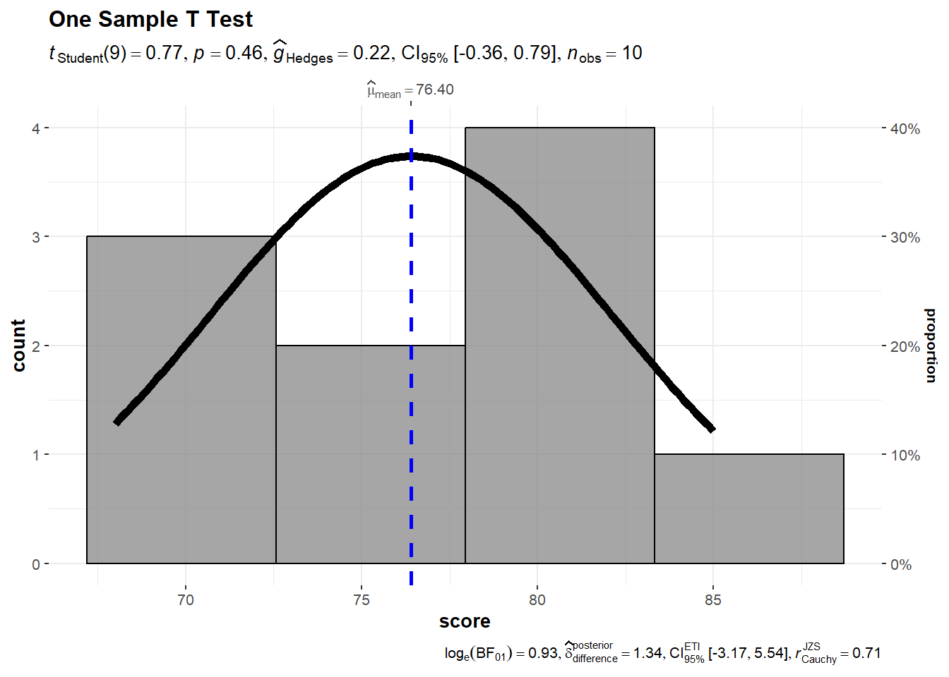
d <- data.frame(score = scores)
gghistostats(
  data = d,#data used
  x = score,# variable of interest
  test.value = 75,# population mean
  type = "parametric",# type of the test for normally distributed data
normal.curve = TRUE
  )+
  labs(title = "One Sample T Test")

Interpretation

Since the p-value (0.171) is greater than the significance level (typically 0.05), we fail to reject the null hypothesis. This means there isn’t enough evidence to conclude that the sample mean is significantly different from the national average of 75.

Conclusion

The one-sample t-test is a powerful statistical tool for comparing a sample mean to a known value. we’ve covered the theoretical background, practical implementation in R, and interpretation of results. Remember to always check the assumptions of normality and independence before performing the test to ensure valid conclusions.