One Way Anova

Published

December 18, 2023

Introduction

Analysis of Variance (ANOVA) is a powerful statistical technique used to compare means across multiple groups. One of the most commonly used forms of ANOVA is the one-way ANOVA, which helps determine whether there are statistically significant differences between the means of three or more independent groups. In this article, we will explore the concept of one-way ANOVA, discuss its importance, and provide a detailed example using R.

What is One-Way ANOVA?

One-way ANOVA is a method used to compare the means of three or more independent groups to see if at least one group mean is different from the others. It extends the t-test to more than two groups and helps avoid the increased risk of Type I error associated with multiple pairwise comparisons.

When to Use One-Way ANOVA?

One-way ANOVA is appropriate when

You have three or more independent groups. The data is continuous and approximately normally distributed within each group. The variances across groups are roughly equal (homogeneity of variances).

Hypotheses in One-Way ANOVA

The one-way ANOVA involves two hypotheses:

Null Hypothesis (H0): All group means are equal

Alternative Hypothesis (H1): At least one group mean is different from the others.

Assumptions of One-Way ANOVA

Normality: The data in each group should be approximately normally distributed.

Independence: The observations in each group should be independent of each other.

Homogeneity of Variances: The variances of the groups should be equal (this can be checked using Levene’s test).

ANOVA Table and F-Statistic

The one-way ANOVA produces an ANOVA table, which includes the following components:

Between-group variability: Variability due to the differences between group means.

Within-group variability: Variability within each group.

F-Statistic: The ratio of between-group variability to within-group variability.

A larger F-statistic indicates a greater likelihood that there is a significant difference between group means.

Example in R

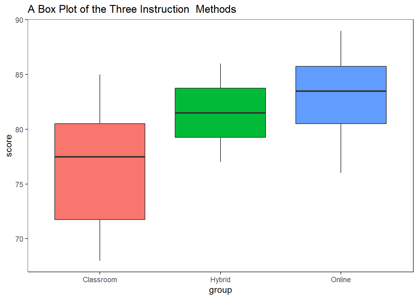
Let’s go through a practical example to understand how to perform a one-way ANOVA in R. Suppose we have three groups of students who received different types of instruction (Classroom, Online, Hybrid), and we want to test if there is a significant difference in their test scores.

Code

# Sample data: students' scores
library(tidyverse)
library(car)
library(ggstatsplot)
library(effectsize)
scores <- data.frame(
  score = c(78, 82, 69, 71, 85, 79, 77, 68, 74, 81, 85, 88, 76, 80, 89, 84, 82, 78, 86, 83, 79, 84, 77, 81, 82, 85, 78, 80, 83, 86),
  group = factor(rep(c("Classroom", "Online", "Hybrid"), each = 10))
)

Code

# checking the assumptions
# normality
scores %>% group_by(group) %>% 
  dlookr::normality(score)

Registered S3 methods overwritten by 'dlookr':
  method          from  
  plot.transform  scales
  print.transform scales

# A tibble: 3 × 5
  variable group     statistic p_value sample
  <chr>    <fct>         <dbl>   <dbl>  <dbl>
1 score    Classroom     0.955   0.732     10
2 score    Hybrid        0.970   0.892     10
3 score    Online        0.974   0.928     10

p-value >.05 indicates that the normality assumptions have been satisfied in all the groups

Code

# homogenity of variance assumptions

leveneTest(score ~ group, data = scores)

Levene's Test for Homogeneity of Variance (center = median)
      Df F value Pr(>F)
group  2     1.8 0.1846
      27

pvalue >.05 indicates that homogenity of variance assumption have been met

Ploting the data

Code

scores %>% 
  ggplot(aes(group, score, fill = group))+geom_boxplot()+
  theme_test()+theme(legend.position = "none")+
  labs(title = "A Box Plot of the Three Instruction  Methods")

Code

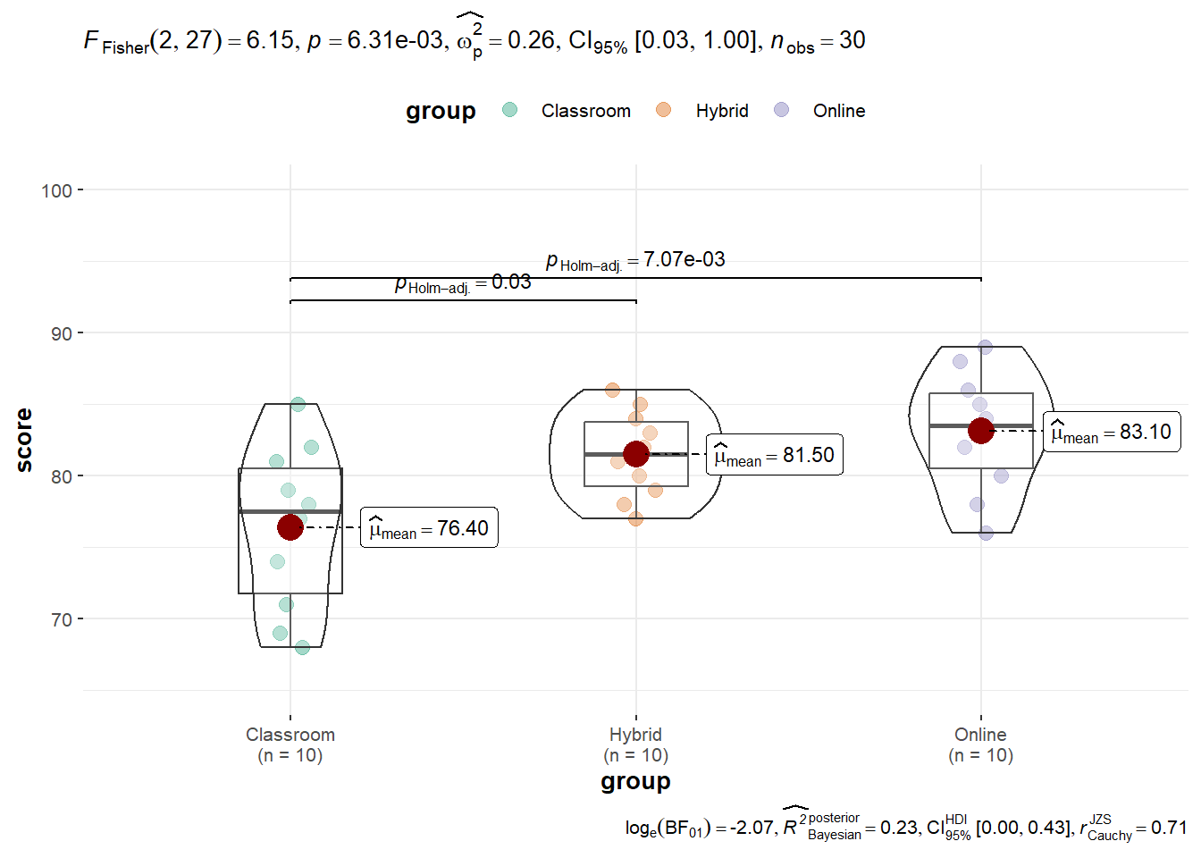
# Perform one-way ANOVA
anova_result <- aov(score ~ group, data = scores)

# Print the result
summary(anova_result)

            Df Sum Sq Mean Sq F value  Pr(>F)   
group        2  244.9  122.43   6.147 0.00631 **
Residuals   27  537.8   19.92                   
---
Signif. codes:  0 '***' 0.001 '**' 0.01 '*' 0.05 '.' 0.1 ' ' 1

Since the p-value (0.00631) is less than the significance level (typically 0.05), we reject the null hypothesis. This means there is enough evidence to conclude that there is a significant difference in test scores between at least one pair of the groups.

Post-Hoc Analysis

If the one-way ANOVA indicates a significant difference, we often conduct a post-hoc analysis to determine which specific groups differ. A common post-hoc test is Tukey’s Honest Significant Difference (HSD) test.

Code

# Perform Tukey's HSD test
tukey_result <- TukeyHSD(anova_result)

# Print the result
print(tukey_result)

  Tukey multiple comparisons of means
    95% family-wise confidence level

Fit: aov(formula = score ~ group, data = scores)

$group
                 diff        lwr       upr     p adj
Hybrid-Classroom  5.1  0.1512763 10.048724 0.0424198
Online-Classroom  6.7  1.7512763 11.648724 0.0064475
Online-Hybrid     1.6 -3.3487237  6.548724 0.7052251

The groups that differs are

Hybrid and Classroom(pvalue = 0.0424198)

Online and classroom(pvalue = 0.0064475)

Visualizing the Test and More Post Hoc Tests

Code

theme_set(theme_test())
ggbetweenstats(
  data = scores,
  x = group,
  y = score,
  type = "parametric",
  var.equal = T
)+ylim(65,100)+theme(legend.position = "top")

Effectsize

Code

interpret_omega_squared(0.26, rules = "cohen1992")

[1] "large"
(Rules: cohen1992)

Cohen (1992) (“cohen1992”) applicable to one-way anova, or to partial eta / omega / epsilon squared in multi-way anova.

ES < 0.02 - Very small

0.02 <= ES < 0.13 - Small

0.13 <= ES < 0.26 - Medium

ES >= 0.26 - Large

The difference is in the three instruction method is large.

Non Parametric Test verson of One Way Anova

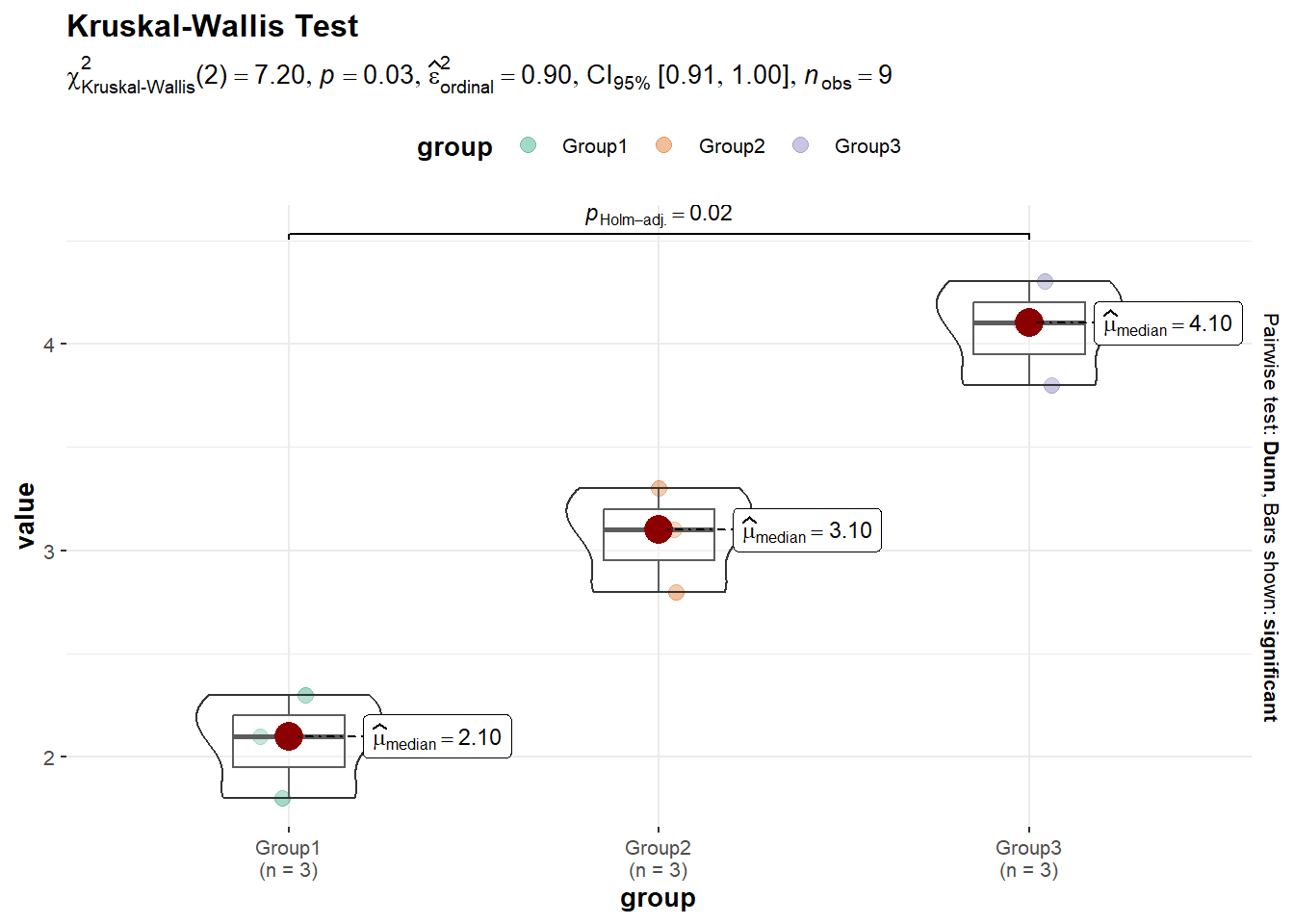
If the data is not normally distributed then we use the non parametric test known as Kruskal-Wallis Test

Example

Code

# Sample data
group1 <- c(2.1, 2.3, 1.8)
group2 <- c(3.1, 3.3, 2.8)
group3 <- c(4.1, 4.3, 3.8)

# Combine data into a data frame
data <- data.frame(
  value = c(group1, group2, group3),
  group = factor(rep(c("Group1", "Group2", "Group3"), each = 3))
)

#Assuming the data is not normally distributed

# Perform the Kruskal-Wallis Test
  
kruskal.test(value ~ group, data = data)


    Kruskal-Wallis rank sum test

data:  value by group
Kruskal-Wallis chi-squared = 7.2, df = 2, p-value = 0.02732

p value <-05 indicates that there is significant difference between the three groups

Kruskal-Wallis Post Hoc Test

Code

library(FSA)

# Perform post hoc pairwise comparisons using the Dunn test
dunn_test_result <- dunnTest(value ~ group, data = data, method = "holm")

print(dunn_test_result)

       Comparison         Z     P.unadj      P.adj
1 Group1 - Group2 -1.341641 0.179712495 0.35942499
2 Group1 - Group3 -2.683282 0.007290358 0.02187107
3 Group2 - Group3 -1.341641 0.179712495 0.17971249

The difference exists in Group 1 and Group 3 only

Visual Format of the Test

Code

ggbetweenstats(
  data = data,
  x = group,
  y = value,
  type = "np"
)+ labs(title = "Kruskal-Wallis Test")+
  theme(legend.position = "top")

Effect size

How much is the difference

Code

interpret_epsilon_squared(0.90)

[1] "large"
(Rules: field2013)

Conclusion

One-way ANOVA is an essential statistical tool for comparing the means of three or more independent groups. Always check the assumptions of normality, independence, and homogeneity of variances before performing the test to ensure valid conclusions.

Understanding and correctly applying one-way ANOVA can significantly enhance your data analysis skills, enabling you to make informed decisions based on your data. Happy analyzing!