Repeated Measure Anova

Published

December 18, 2023

Introduction

Repeated Measures ANOVA (Analysis of Variance) is a statistical technique used when the same subjects are measured multiple times under different conditions. This method is particularly useful in experimental designs where the same participants are exposed to various treatments or conditions.

What is Repeated Measures ANOVA?

Repeated Measures ANOVA is an extension of the traditional ANOVA used when the same subjects are involved in more than one treatment condition. It helps determine whether there are significant differences between the means of different conditions, taking into account the correlation between repeated measurements on the same subjects.

When to Use Repeated Measures ANOVA?

The same subjects are measured under different conditions or at different time points.

The data is continuous and approximately normally distributed.

The measurements are correlated within subjects.

Hypotheses in Repeated Measures ANOVA

Null Hypothesis (H0): The means of the different conditions are equal

Alternative Hypothesis (H1): At least one condition mean is different from the others.

Advantages of Repeated Measures ANOVA

Increased Power: Since the same subjects are used in all conditions, the variability due to individual differences is reduced, leading to higher statistical power.

Efficiency: Fewer subjects are required compared to a between-subjects design.

Control for Individual Differences: By measuring the same subjects under different conditions, individual differences are controlled.

Assumptions of Repeated Measures ANOVA

Normality: The data within each condition should be approximately normally distributed.

Sphericity: The variances of the differences between all pairs of conditions should be equal (this can be checked using Mauchly’s test).

Independence: The observations within each condition should be independent of each other.

Example in R

Let’s go through a practical example to understand how to perform Repeated Measures ANOVA in R. Suppose we have a study where the same group of students is tested on their math scores after using three different study methods (Traditional, Online, Hybrid).

Code

library(tidyverse)# data manipulation
library(ggstatsplot)# visualizing and conducting statistical tests
library(car)#homogenity of variance
library(rstatix)#Perform the Repeated Measures ANOVA 
library(effectsize)
# Sample data: students' scores
data <- data.frame(
  subject = factor(rep(1:10, each = 3)),
  method = factor(rep(c("Traditional", "Online", "Hybrid"), times = 10)),
  score = c(67, 80, 84, 71, 76, 85, 77, 83, 90, 81, 84, 88, 76, 80, 89, 80, 83, 86, 81, 83, 88, 72, 84, 80, 78, 87, 84, 80, 86, 90))

Assumption of normality

Code

#shapiro wilk test
data %>% 
  group_by(method) %>% 
  dlookr::normality(score)

# A tibble: 3 × 5
  variable method      statistic p_value sample
  <chr>    <fct>           <dbl>   <dbl>  <dbl>
1 score    Hybrid          0.922   0.376     10
2 score    Online          0.929   0.438     10
3 score    Traditional     0.885   0.147     10

Normality Assumption is met as p value is greater than 0.05

Conducting the Test

Method1

Code

# Perform Repeated Measures ANOVA
anova_result <- aov(score ~ method + Error(subject/method), data = data)

# Print the result
summary(anova_result)


Error: subject
          Df Sum Sq Mean Sq F value Pr(>F)
Residuals  9  245.4   27.26               

Error: subject:method
          Df Sum Sq Mean Sq F value   Pr(>F)    
method     2  520.5   260.2   31.75 1.25e-06 ***
Residuals 18  147.5     8.2                     
---
Signif. codes:  0 '***' 0.001 '**' 0.01 '*' 0.05 '.' 0.1 ' ' 1

since the p-value (<.001) is less than the significance level (typically 0.05), we reject the null hypothesis. This means there is enough evidence to conclude that there is a significant difference in math scores between at least one pair of study methods.

Method2

Code

# Perform the Repeated Measures ANOVA 
anova_result2 <- data %>% anova_test(dv = score, wid = subject, within = method)

Assumption of sphericity

Method1

Code

anova_result2$`Mauchly's Test for Sphericity`

  Effect     W    p p<.05
1 method 0.968 0.88

The Mauchly’s Test of Sphericity gives a Mauchly’s W test statistic of .968, p > .05. We can therefore conclude that the sphericity assumption has been met

Method2

Code

anova_result2$`Sphericity Corrections`

  Effect   GGe      DF[GG]    p[GG] p[GG]<.05   HFe      DF[HF]    p[HF]
1 method 0.969 1.94, 17.45 1.75e-06         * 1.231 2.46, 22.16 1.25e-06
  p[HF]<.05
1         *

However, some debate as to the sensitivity of Mauchly’s test in its ability to detect sphericity. There is therefore the alternative of consulting the Epsilon value quoted in the Greenhouse-Geisser column. This figure should be as close to 1.00 as possible in order to indicate no sphericity problems. Our value is .969 so we can be confident that issues of sphericity do not affect our calculations

Method3

Code

## spericity
data$method <- factor(data$method)
data_s <- data %>% 
  pivot_wider(names_from = "method", values_from = "score")
data_s %>% mutate(
  trad_onl =(Traditional- Online), trad_hyb = (Traditional-Online),
  onl_hyb = (Online-Hybrid)) %>% 
  data.frame() %>% 
  select(-2,-3,-4) %>% 
  pivot_longer(cols = c(2,3,4), names_to = "differences", values_to = "score_d") %>% 
  group_by(differences) %>% 
  leveneTest(score_d ~differences, data = .)

Levene's Test for Homogeneity of Variance (center = median)
      Df F value Pr(>F)
group  2  0.0047 0.9953
      27

p value >.05 indicates equal variances of differences between all possible pairs of conditions thus the sphericity assumption have been met.

Code

anova_result2$ANOVA

  Effect DFn DFd     F        p p<.05  ges
1 method   2  18 31.75 1.25e-06     * 0.57

since the p-value (<.001) is less than the significance level (typically 0.05), we reject the null hypothesis. This means there is enough evidence to conclude that there is a significant difference in math scores between at least one pair of study methods.

Post-Hoc Analysis

Code

# Perform pairwise comparisons with holm correction
pairwise.t.test(data$score, data$method, p.adjust.method = "holm",
                paired = T)


    Pairwise comparisons using paired t tests 

data:  data$score and data$method 

            Hybrid  Online
Online      0.0230  -     
Traditional 5.5e-05 0.0011

P value adjustment method: holm

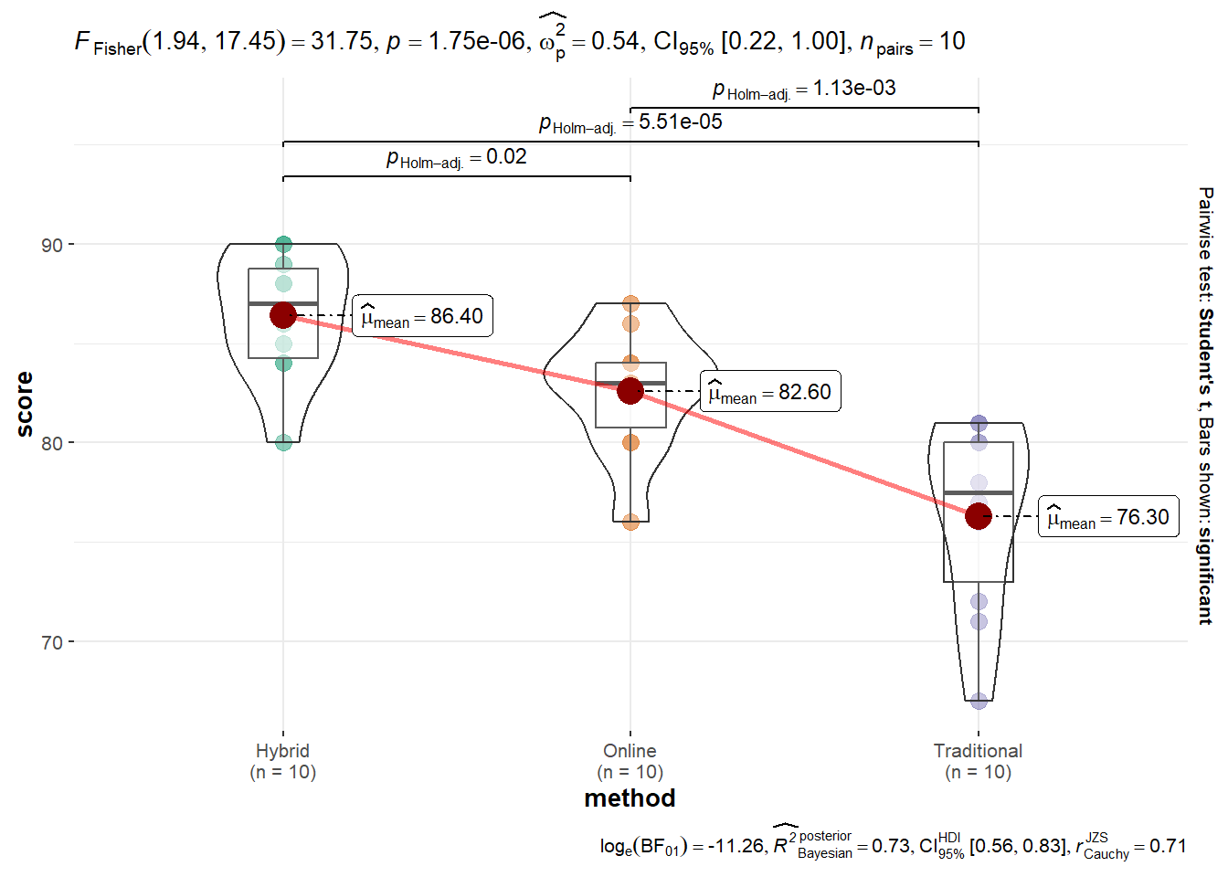
All the three Methods differs with hybrid method having the highest scores

Visual Format of the Test

Code

ggwithinstats(
  data = data,
  x = method,
  y = score,
  type = "p"
)

Effectsize

Code

interpret_omega_squared(0.54,rules = "cohen1992" )

[1] "large"
(Rules: cohen1992)

The difference between the three methods is large

Non Parametric test

Friedman Test

The Friedman Test is a non-parametric test used to detect differences in distributions across multiple related samples. It serves as an alternative to repeated measures ANOVA.

Example in R

lets see whether the advertisement methods differs in the profit yielded by a company the advertisement method are youtube,facebook and newspaper from the marketing data from datarium package

Code

# Sample data
library(datarium)
data <- marketing %>% 
  select(youtube,facebook,newspaper) %>% 
  pivot_longer(cols = 1:3,names_to =  "channel",
               values_to = "money") %>% 
  mutate(id = rep(1:200, each =3))
  
# Perform the Friedman Test
t <- friedman_test(money ~ channel | id, data = data)
t

# A tibble: 1 × 6
  .y.       n statistic    df        p method       
* <chr> <int>     <dbl> <dbl>    <dbl> <chr>        
1 money   200      190.     2 6.07e-42 Friedman test

Code

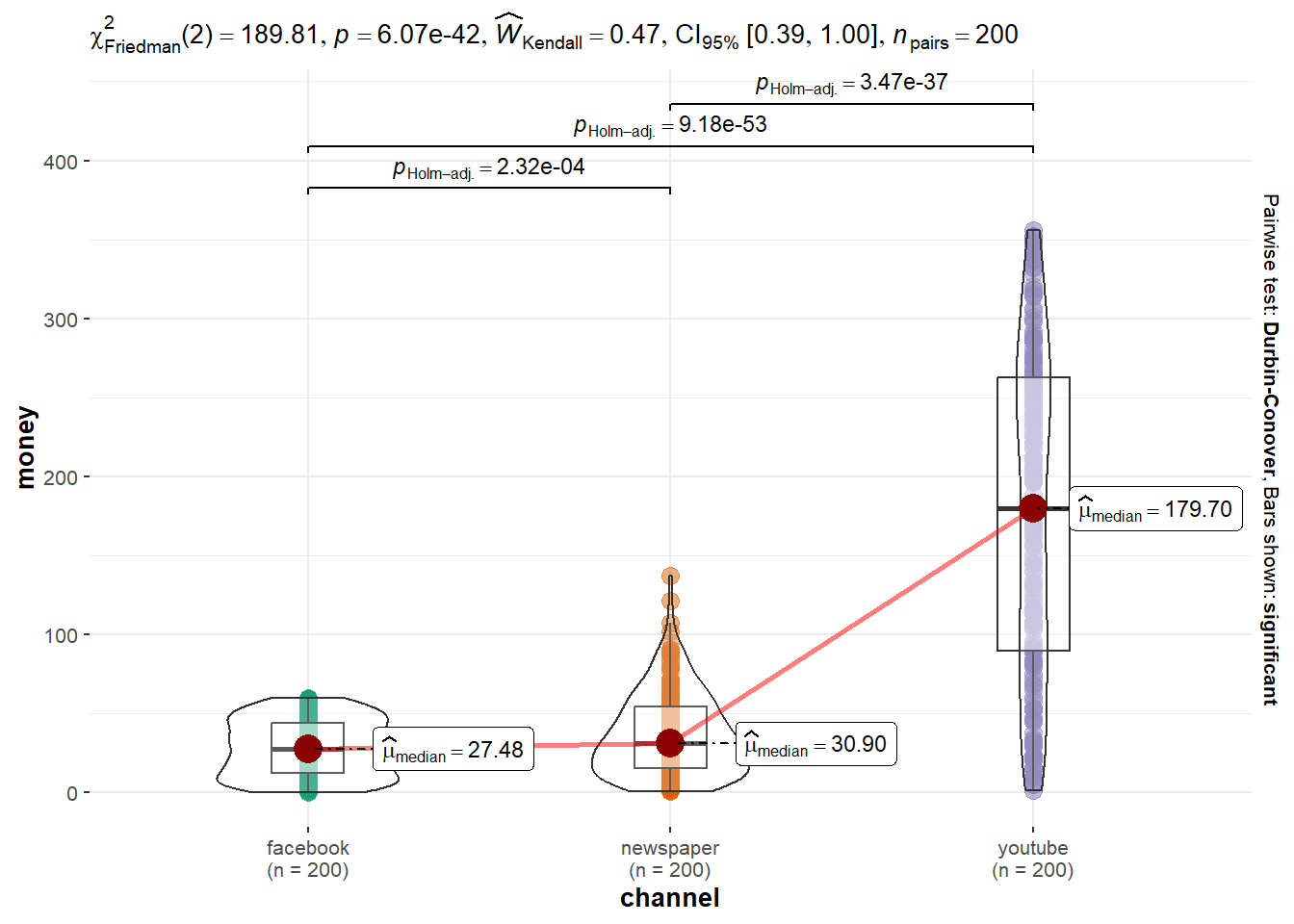
ggwithinstats(
  data = data,
  x = channel,
  y = money,
  type = "np"
)

Effectsize

Code

interpret_kendalls_w(0.47)

[1] "moderate agreement"
(Rules: landis1977)

The three advertising methods differs significantly and the different is moderate

conclusion

Repeated Measures ANOVA is a crucial statistical tool for analyzing data from experiments where the same subjects are measured under different conditions. In this article, we’ve covered the theoretical background, practical implementation in R, and interpretation of results. Always check the assumptions of normality, sphericity, and independence before performing the test to ensure valid conclusions.