Chi Square Test

Introduction

The Chi-Square test is a non-parametric statistical technique used to examine the association between categorical variables. It is widely used in various fields, from social sciences to medical research, to test hypotheses about relationships between categorical data.

What is the Chi-Square Test?

The Chi-Square test assesses whether there is a significant association between two categorical variables. It compares the observed frequencies in each category to the expected frequencies under the null hypothesis of no association.

Types of Chi-Square Tests

Chi-Square Test of Independence

Tests whether two categorical variables are independent of each other.

Chi-Square Goodness-of-Fit Test

Tests whether the distribution of a single categorical variable matches an expected distribution.

When to Use the Chi-Square Test?

The data is categorical.

You want to test the association between two categorical variables (for the test of independence) or compare observed frequencies to expected frequencies (for the goodness-of-fit test).

The sample size is sufficiently large (expected frequencies should generally be 5 or more in each category).

Hypotheses in Chi-Square Test of Independence

Null Hypothesis (H0): The two categorical variables are independent.

Alternative Hypothesis (H1): The two categorical variables are not independent.

Assumptions of Chi-Square Test

Independence: The observations should be independent of each other.

Expected Frequency: The expected frequency in each category should be at least 5.

Example in R

Let’s go through a practical example to understand how to perform a Chi-Square test of independence in R. Suppose we have data on the smoking habits of different age groups and we want to test if there is an association between age group and smoking status.

Code

# Sample data: smoking habits of different age groups
age_groups <- c("18-25", "26-35", "36-45", "46-55", "56+")
smoking_status <- c("Smoker", "Non-Smoker")
data <- matrix(c(25, 75, 50, 50, 30, 70, 20, 80, 10, 90), nrow = 5, byrow = TRUE)
colnames(data) <- smoking_status
rownames(data) <- age_groups

# Perform Chi-Square test of independence
chi_square_test <- chisq.test(data)

# Print the result
print(chi_square_test)

    Pearson's Chi-squared test

data:  data
X-squared = 44.647, df = 4, p-value = 4.707e-09

Since the p-value (<.001) is less than the significance level (typically 0.05), we reject the null hypothesis. This means there is enough evidence to conclude that there is a significant association between age group and smoking status.

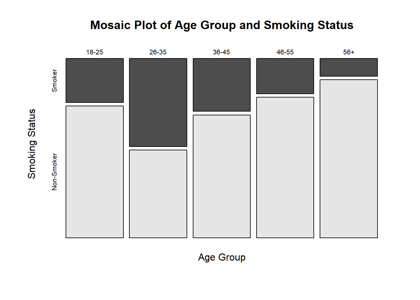
Visualizing the Data

Visualizations can help us understand the data distribution and support our findings.

Code

# Mosaic plot
mosaicplot(data, main = "Mosaic Plot of Age Group and Smoking Status", xlab ="Age Group",
             ylab ="Smoking Status" , color = TRUE)

Chi-Square Goodness-of-Fit Test

Example

Let’s also go through a practical example to understand how to perform a Chi-Square goodness-of-fit test in R. Suppose we have data on the color distribution of candies in a bag and we want to test if the distribution matches an expected distribution.

Code

# Sample data: color distribution of candies
observed <- c(50, 30, 20)
expected <- c(40, 40, 20)

# Perform Chi-Square goodness-of-fit test
chi_square_gof <- chisq.test(observed, p = expected/sum(expected))

# Print the result
print(chi_square_gof)

    Chi-squared test for given probabilities

data:  observed
X-squared = 5, df = 2, p-value = 0.08208

Since the p-value (0.08208) is greater than the significance level (typically 0.05), we fail to reject the null hypothesis. This means there is not enough evidence to conclude that the color distribution of candies significantly differs from the expected distribution.