Correlation Test

Published

December 19, 2023

Introduction

Correlation is a statistical measure that describes the extent to which two variables change together. In other words, it quantifies the degree of relationship or association between two continuous variables. Correlation does not imply causation, but it indicates the strength and direction of a linear relationship between variables.

Types of Correlation

Positive Correlation

When one variable increases, the other variable tends to increase as well. Represented by a correlation coefficient

r between 0 and 1.

Negative Correlation

When one variable increases, the other variable tends to decrease. Represented by a correlation coefficient

r between 0 and -1.

No Correlation (Zero Correlation):

There is no systematic relationship between the variables. Represented by a correlation coefficient

r close to 0.

Interpretation of Correlation

Strength:

The closer r is to 1, the stronger the correlation. Values around 0.8 or -0.8 and above are considered strong correlations.

Direction:

The sign of r indicates the direction of the correlation. Positive r indicates a positive correlation, and negative r indicates a negative correlation. Cautions:

NOTE

Correlation does not imply causation.
Outliers can influence correlation.
Non-linear relationships may not be captured.

Example of Exploratory Analysis Using Correlation

Required Packages

Code

library(tidyverse)
library(psych)
library(dlookr)

Lets perfoming exploratory data analysis using Iris dataset in r

Code

head(iris)

  Sepal.Length Sepal.Width Petal.Length Petal.Width Species
1          5.1         3.5          1.4         0.2  setosa
2          4.9         3.0          1.4         0.2  setosa
3          4.7         3.2          1.3         0.2  setosa
4          4.6         3.1          1.5         0.2  setosa
5          5.0         3.6          1.4         0.2  setosa
6          5.4         3.9          1.7         0.4  setosa

Correlation Analysis

Code

plot_correlate(iris[,-5])

Warning: 'plot_correlate' is deprecated.
Use 'plot.correlate' instead.
See help("Deprecated")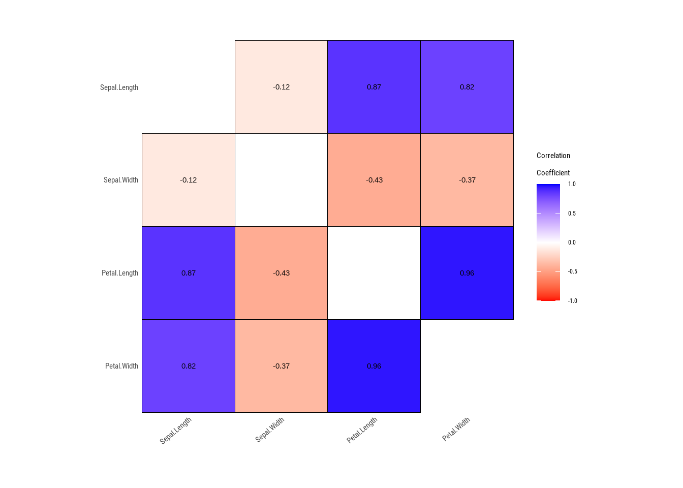

The above correlation matrix shows correlation between variables in the dataset. However, deriving conclusion from plain correlation can lead to wrong conclusion. Its better to visualize the data together with its correlation for better results.

Code

PerformanceAnalytics::chart.Correlation(iris[,-5])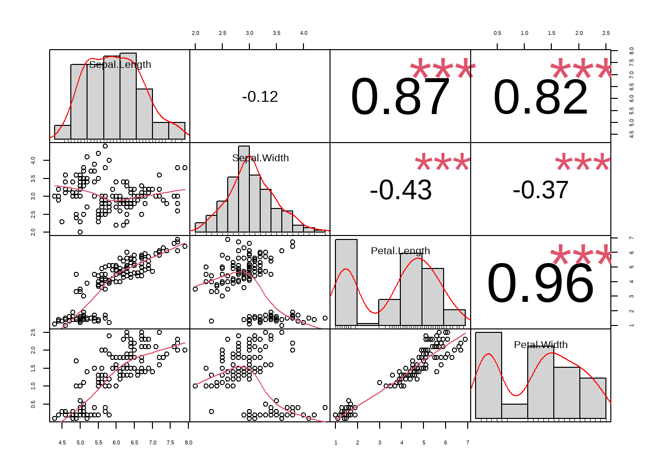

The plot shows correlation together with the significance level.

From the plot we can uncover three things

The data is not linear as it can be seen from the scatter plot(correlation only make sense when the data is linear)
The data is clustered into three groups and generalizing correlation for all groups might be wrong. lets look correlation for each group

Code

GGally::ggpairs(iris,
                columns = 1:4,
                aes(colour = Species),
                lower = list(continuous = "smooth"))

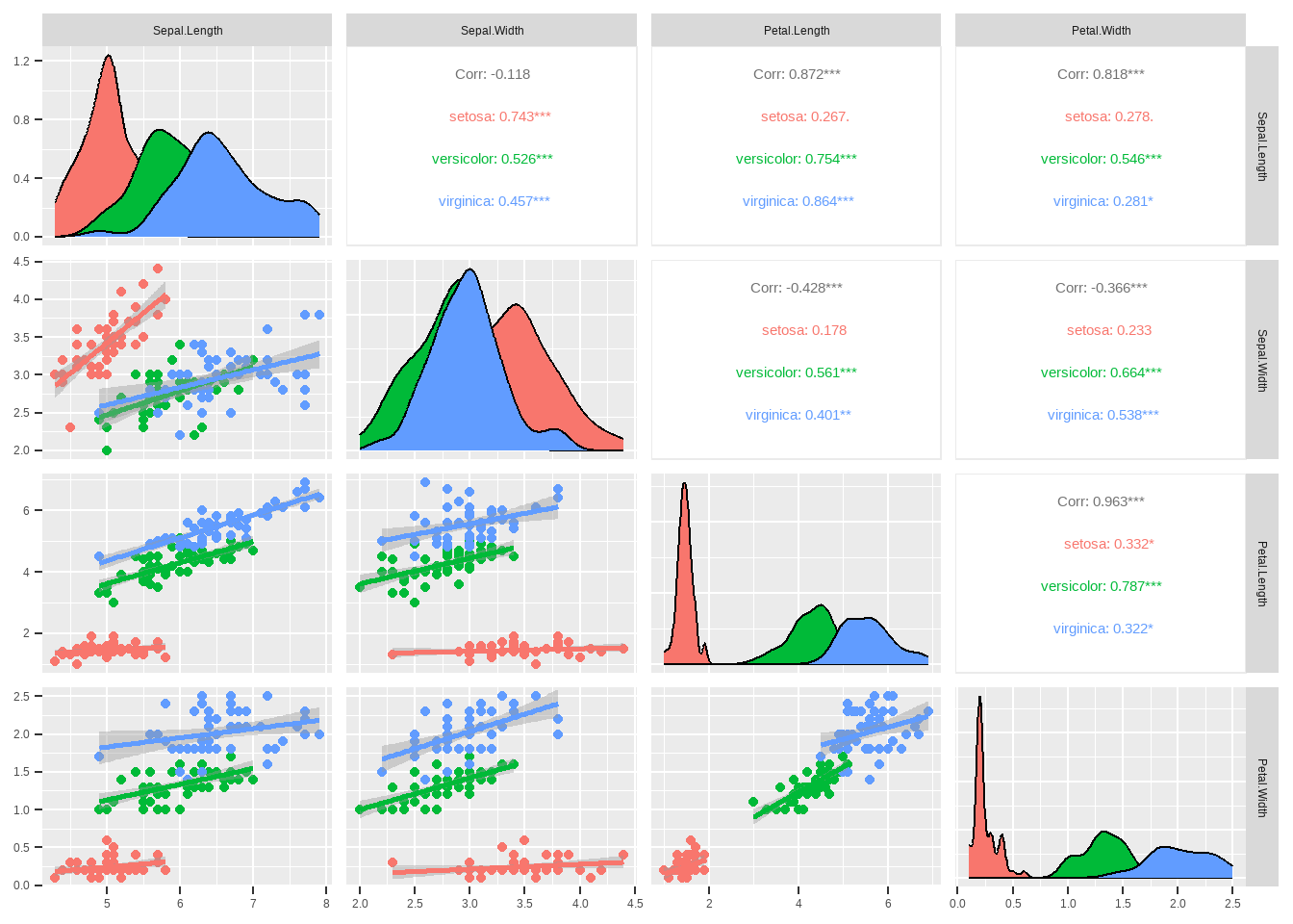
Two of the negative correlation between 2 groups shows the opposite of what is actually true.

The correlation between sepal.Length and sepal.Width which is generalized as -0.118 and not significant is wrong. The truth is the correlation is positive and significant for each group.

The correlation between petal.Length and sepal.Length is generalized as 0.872(significant). However,it is not true for group Setosa whose correlation of the same variables is 0.267 and insignificant. Accepting the generalized correlation can lead to type two error(Missing a discovery) or type one error for variables Petal.Lenth and Sepal.Width whose generalized correlation is negative and significant(-0.428). However,for setosa the correlation is positive and not significant.

The normality of the data as it can be seen from the density plot.

Discovering the normality of the data helps to decide which type method of correlation to use parametric or non parametric. To confrim this we can use shapiro wilk test to test the normality of each group

Code

iris %>% 
  group_by(Species) %>% 
  normality()  %>% 
  flextable::regulartable()

variable	Species	statistic	p_value	sample
Sepal.Length	setosa	0.9776985	0.4595131518060	50
Sepal.Length	versicolor	0.9778357	0.4647370392777	50
Sepal.Length	virginica	0.9711794	0.2583147454315	50
Sepal.Width	setosa	0.9717195	0.2715263939044	50
Sepal.Width	versicolor	0.9741333	0.3379951082610	50
Sepal.Width	virginica	0.9673905	0.1808960403668	50
Petal.Length	setosa	0.9549768	0.0548114671464	50
Petal.Length	versicolor	0.9660044	0.1584778383480	50
Petal.Length	virginica	0.9621864	0.1097753694872	50
Petal.Width	setosa	0.7997645	0.0000008658573	50
Petal.Width	versicolor	0.9476263	0.0272778041408	50
Petal.Width	virginica	0.9597715	0.0869541879469	50

higher p value means that the data is normally distributed. Therefore we should use parametric pearson correlation. however if we generalized the data the result would be

Code

iris %>% 
  normality() %>% 
  flextable::regulartable()

vars	statistic	p_value	sample
Sepal.Length	0.9760903	0.0101811611756293	150
Sepal.Width	0.9849179	0.1011542684359037	150
Petal.Length	0.8762681	0.0000000007412263	150
Petal.Width	0.9018349	0.0000000168046517	150

Some lower p values indicates that the data is not normally distributed.

Therefore we might have ended up using non parametric test which is wrong in this case